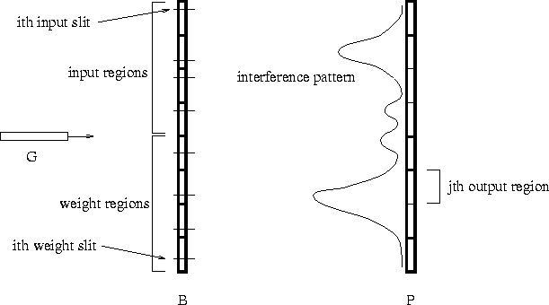
Figure 1: A feed-forward quantum neurocomputer. See text for key.
Hopfield [Hopfield, 1982] popularized the idea that any physical dynamical system could be constrained to serve as a neural network, with fixed points of the system acting as ``memories'', which could be recalled associatively, in a content-addressable manner. However, the learning algorithms availble for the attractor-based neural networks on which Hopfield focussed are not as powerful as those for feed-forward networks, for which Hopfield's observation also applies. It is for this reason, and because the feed-forward back-propagation network is the one most likely to be familiar to a general audience, that the exmaple here will be based on a feed-forward network architecture. The principles and insights, however, generalize to other kinds of neural network.
Similarly, many different quantum situations could be used to implement a learning algorithm; I will stick to the situation of a barrier with slits in front of a photo-sensitive plate, because of its familiarity. It is very likely that such a situation would prove impractical in order to obtain some of the computational advantages (especially those of speed and size) of quantum computing, but as such advantages are relatively obvious, and are not the advantages on which I will be concentrating, this impracticality need not concern us much.
The details of feed-forward networks involve units, activation values, layers, and weights. But what is important at first is that:

Figure 1: A feed-forward quantum neurocomputer. See text for key.
A quantum implementation of this kind of network is illustrated in figure 1. A particle beam G is set up facing a barrier B, behind which is a photo-sensitive plate P. The barrier has several slits in it, which are responsible for the famous interference patterns on the plate. Some of the slits are designated to be input slits, and the rest are the weight slits. The interference pattern on the plate P that results from the beam G being aimed at the barrier B with a particular input slit configuration is the output of the system for that input. Thus, use of the system to perform some computation will require two mappings: one (I) from inputs (e.g., character strings, images, queries, etc.) to input slit configurations, and one (O) from interference patterns to outputs (e.g., classifications, stored data, etc.).
Assume that one already has a mapping from inputs to n-vectors, and a mapping from m-vectors to outputs. One could map these input n-vectors to input slit configurations by, for example, dividing the barrier into n sections, each having an input slit, with the relative position of the ith slit within the ith section of the barrier indicating the value of the ith coordinate of the input vector (this is the type of arrangement depicted in figure 1). For binary input vectors, this mapping could be even simpler: there is a slit in the nth section of the barrier if and only if the nth coordinate of the input vector is ``1''.
Less straightforward is the mapping O from interference patterns to outputs. Since interference patterns are of high-dimensionality, any dimension-reducing mapping will do. Perhaps the plate could be divided into m sections, and the average intensity within the mth region can serve as the mth coordinate of the output vector. For the case of binary output vectors, a soft (sigmoid) thresholding of this value would do (the thresholding must be soft so as to allow differentiation for back-propagation learning; see below).
The error of the system, E, is defined to be some function of
the desired ( ![]() ) and actual (
) and actual ( ![]() ) output vectors, typically
) output vectors, typically
![]() . If
. If ![]() is the function that yields
an interference pattern
is the function that yields
an interference pattern ![]() given an input
given an input ![]() and a weight slit
configuration
and a weight slit
configuration ![]() , then
, then ![]() .
.
Given some such setup, the system could learn an associative mapping f in the following way:
After several passes through the training set, this procedure will ensure that the system settles into a weight configuration that produces minimal error on the training set. In many cases, this will also result in good performance on other samples drawn from the same source as the training set (i.e., generalization).
This is enough to establish a correspondence between neural nets and a quantum system. The correspondence can then be used to suggest how the many variations on connectionist learning (e.g., recurrency, competitive learning, etc.) also could be implemented in a quantum system.