References.

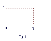
Vectors.

Sometimes it is much more convenient to group numbers that have common attributes and treat them like one. Take for example the co-ordinates of a single point in the 2D space (fig 1). Instead of having two separate numbers to describe the point, we use a vector (3,2), which describes its position.

A vector is 1-dimensional structured collection of numbers that may have either of the following forms:

Matlab supports vectors and you only have to type [3,2] or [3;2] respectively to enter vectors a and b. We say that the dimensions of vector a are 1x2 (one row, two columns) and the dimensions of vector b are 2x1 (two rows, one column).

The arithmetic operations +, -, * , / can be applied to vectors:

Addition between two vectors simply means adding each element of one vector to the corresponding element of the other:

[ 3 2 ] + [ 5 7 ] = [ 8 9 ]

since 3+5=8 and 2+7=9. Of course vectors should be of the same dimensions (here 1x2).

Addition between a vector and a number in Matlab will result in adding the number to each element of the vector:

>> a=[1 2];
>> a+1

ans =

   2 3

Subtraction is similar to addition:

>> [3 2] - [5 7]

ans =

   -2 -5

In vector cases, however, we may have two kinds of multiplication: "point to point" multiplication and true vector multiplication.

Point to point multiplication ( operator .* ) is as simple as addition and subtraction:

>> [3 2] .* [5 7]

ans =

   15 14

since 3*5=15 and 2*7=14.

Vector multiplication (operator *) is a bit more complicated. In this case the vectors should not be of the same dimensions but they need to have some sort of relation:

If the dimensions of vector a are 1x2 then the dimensions of vector b should be 2x1 in order to multiply them. In other words the number of columns of the first vector should be the same as the number of rows of the second vector. The result will be a vector of dimensions 1x1 (single element).

You can also multiply a vector with a simple scalar (using either .* or * the result will be the same). Such an operation will result in a vector where every element is multiplied with the number:

>> a=[3 5];
>> 5*a

ans =

   15 25

>> 5.*a

ans =

    15 25

Point to point division ( operator ./ ) can be defined between a number and a vector or a vector and a vector in a similar way to point to point multiplication:

>> b=[2 10];
>> a=[1 2];
>> b./a

ans =

    2 5

>> b./2

ans =

1 5

Division between vectors is not defined.

A vector to the power of a number will have as a result a new vector whose elements will be the elements of the previous one at that power. Here the operator is .^, similar to the previous cases. In Matlab basic functions like cos and exp are designed taking into account that the input argument could be a vector. Therefore cos or exp with input argument a vector will have as a result a vector of the same dimensions, each element of which will be the cosine or exponential of the corresponding element of the original vector.

>> x=[1:0.5:3]

x =

    1.0000 1.5000 2.0000 2.5000 3.0000

>>exp(x)

ans =

    2.7183 4.4817 7.3891 12.1825 20.0855

1. Suppose that x takes on the values x=1, 1.1, 1.2 ,1.3...10. Create a vector named x with these values and define y=cos(2*x). Find more about the plot command and use it to plot x,y. Note: you may find it useful to use the colon (:) operator.

2. Modify the sigmoid function that you created in lab 1 (exercise 10) to accept a vector as input argument.

3. In a simple neural network (like the one we came across in the previous lab) we can write the inputs and the weights in vector form. You can easily prove that:

   

   where w is a vector 1x3 containing the weights and x is a vector 3x1 containing the 3 inputs. Apparently w1 will be the first element of w and x1 the first element of x. Show the above equality (written).

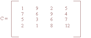
Matrices.

In many cases, we need to address problems more complicated than this network. There is a more general form than vectors that can be used in such cases, called a matrix. A matrix has the following form:

And we can refer to an element separately by using the number of the row and column to which it belongs. For example 27 belongs to row 3 column 5, therefore we can refer to it: A_3,5.

To enter matrix A into Matlab:

>> A=[ 3 6 8 9 12; 4 14 5 17 2; 1 7 15 11 27]

A =

  3   6    8    9   12
  4  14   5  17   2
  1   7  15  11  27

>> A(3,5)

ans =

27

Operations on matrices are similar to vector operations. For example addition:

>> B=[ 1 2 3; 4 5 6]

B =

    1   2   3
    4   5   6

>> C=[ 13   5   72;   0   -3   7]

C =

13   5   72

 0   -3   7

>> B+C

ans =

   14   7   75
    4   2   13

There is also "point to point" multiplication and division for matrices. The only operation that is slightly more complicated is true matrix multiplication. The same rule applies here as well: The number of columns of the first matrix should be the same as the number of rows of the second matrix. The result of such a multiplication is a matrix (R) with rows the number of rows of the first matrix and columns the number of columns of the second matrix. Element R_1,2 of the matrix will be calculated by taking the 1st row of the first matrix and multiply it with the 2nd column of the second matrix. Note that a single row or a single column of a matrix is a vector. Therefore, to calculate each element of the matrix R, you have to make one vector multiplication. In general, to calculate element R_m,n you need to multiply the m row of the first matrix with the n column of the second matrix. An easy way to calculate all the elements is first to pre-decide the dimensions of the matrix to be calculated and then multiply the 1st row of the first matrix with the 1st column of the second and write it as element R_1,1, then the 1st row of the first matrix with the 2nd column of the second and write the result as element R_1,2 etc till you finish with all the columns of the second matrix. Then go to the second row of the first matrix and do the same till you finish with all rows of the first matrix.

Matlab will do this for you, faster.

>> A=[ 1 2 3; 1 2 2]

A=

   1   2   3
   1   2   2

>> B=[ 2 3 2; 4 1 2; 0 0 1]

B =

   2   3   2
   4   1   2
   0   0   1

>> A*B

ans =

   10   5   9
   10   5   8

4. Verify (handwritten) the result of the above multiplication.

5. Create the matrix C. Find more about the colon operator by using the help command or the Helpdesk. Display column 1 of matrix C. Display columns 2 to 3. Display row 4. Display elements 2 to 4 of the 3rd row. Find about the command sum and apply it to the matrix C. Use the ' operator to transpose the matrix (syntax: C').

   

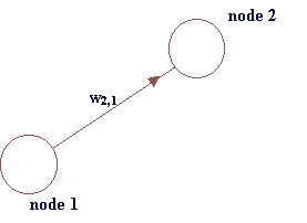
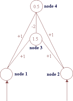
In neural networks matrices are quite useful, as there are cases where we have to deal with complex structures. When we have to deal with a network with more than one layer, like the one in the next exercise, we may need a matrix to store the weight values instead of a simple vector. In this case, we use the following notation: We set up a matrix W and store the weights in such a way that for example w_2,1 is the weight from node 1 to node 2. If there is no such weight, we put 0 instead.

6. A multi-layer network consists of 4 units. Units 1 and 2 are input units, unit 3 is a hidden unit and unit 4 is an output unit. Create a vector A to contain the values of the input, hidden and output units. Set up the associated weight matrix (W 4x4) as an array structure with W(3,1)=1, W(3,2)=1, W(4,1)=1, W(4,2)=1 and W(4,3)=-2, otherwise W(i,j)=0. Hidden unit 3 has a threshold function at 1.5 and output unit 4 at 0.5. You should be in a position to verify that the following image represents the structure of the network:

   

   Write down the expressions that will lead you to the calculation of the network output, by using the matrices you have already defined. To do this, set the activation values for units 1 and 2, then calculate the netinput for unit 3 by vector matrix multiplication (vector A with row 3 of matrix W). Then use the threshold function for this unit and set the activation of unit 3. Repeat the calculation for unit 4, finding the netinput (with which row do you have to multiply vector A to calculate netinput for unit 4?) then thresholding and setting the activation. The value of unit 4 is now returned as the final output of the network. Test the networks for all possible inputs (0 or 1). The output of the network should be the XOR function.

7. Redesign the neural network that implements the AND function by using vectors/matrices (exercise 3) including the training process (linear delta rule). You may use a 3x4 matrix to store the input values, a 1x4 row vector to store the targets and a 1x3 row vector to store the weights.