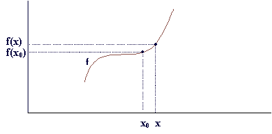
Warning: You should complete lab1 before attempting to deal with lab2 and have finished lab2 before dealing with coursework 1.

PART 1: DIFFERENTIATION.

Definition: Consider the following function f(x), a point x₀ of the x axes and any other point x close to x_0.

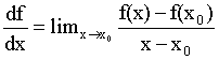
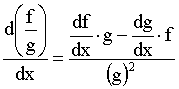
The first derivative of the function f at the point x₀ is defined as:

where the symbol lim_x->x0 means that points x and x₀ are very close to each other. In practice we never use this definition to calculate the derivative of a function. What we do is learn the derivatives of some basic functions and the derivative rules and combine them to calculate the derivatives of some more complicated functions. The derivatives of the basic functions have -of course- been calculated by using the definition of the derivative. Though you might never use this definition yourself, you will probably find it useful to keep in mind what the derivative is all about.

First of all the derivative of a function is another function which gives us important knowledge about the initial function. For example if your function is increasing around a certain point x₀, f(x) will be greater than f(x₀) therefore the numerator will be positive. The denominator will also be positive which means that the derivative at x₀ will be a positive number. This number shows how the function is changing if you make a small change at x.

When we want to refer to the derivative of a one variable function f(x) in general we can use the symbols df/dx , df(x)/dx or f ^´(x) but when we discuss the value of the derivative at a particular point x₀ we will use the symbol df(x₀)/dx or f ^´(x₀). Note that x₀ can be any number, where the original function is defined.

Another symbol often used to describe the difference between two values of a variable is the Greek letter delta, equivalent of D :

Examples:Assume that you have to deal with the very simple function f(x)=x :

1. Plot the function f(x)=x on Matlab. Type:

   >>x=linspace(0,10,10);
   >>y=x;
   >>plot(x,y);

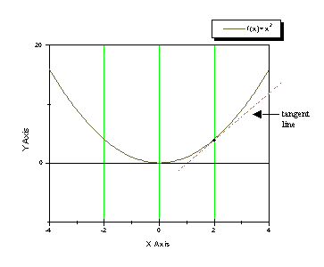
The first derivative at any point x₀ is 1, which means the function is increasing in the same way at any point.

Another example is the first derivative of f(x)=x². In this case f´(x)=2x. The derivative at x=2 equals to: f´(2)=2*2=4 . That means that, near the point x=2, the function f(x)=x² is increasing. The derivative df/dx=4 is equal to the slope of the tangent line of the function at x=2. If we calculate the derivative at x=-2 is f´(-2)= 2*(-2)=-4, which shows that the function is decreasing around x=-2.

2. Plot the function f(x)=x² in Matlab. Type:

   >>x=linspace(-4,4,30);
   >>y=x.^2;
   >>plot(x,y)

First derivative of some basic functions.

• Constant function f(x) = c --- f ´(x) = 0
  e.g. f(x)=5 --- f ´(x) = 0

• f(x)=x --- f ´(x)= 1

• f(x)= x^a --- f ´(x)= ax^a-1
  e.g. f(x)=x⁵ --- f ´(x)= 5x⁴

• f(x)=sin(x) --- f ´(x)= cos(x)

• f(x)=cos(x) --- f ´(x)= -sin(x)

• Logarithmic function f(x)=log(x) --- f ´(x)= 1/x

• Exponential function f(x)= e^x --- f ´(x)=e^x

3. Plot the function f(x)=log(x) and its first derivative in Matlab. Type:

   >>x=linspace(1,4,30);
   >>y=log(x);
   >>plot(x,y,'b')
   >>hold on
   >>z=1./x;
   >>plot(x,z,'y')

Derivative rules.

• Addition and Subtraction.
  The derivative of the addition (or subtraction) of two functions is equal to the derivative of the first function plus (or minus) the derivative of the second function.

  

  Examples:
  f(x)=x²+3: We can consider it an addition of two functions, f₁(x)=x² and f₂(x) =3. We know that f₁´(x)=2x and that f₂´(x)=0 (constant function). Therefore f´(x)=2x.

  f(x)=e^x-x+7: This function is an addition of 3 known functions. The rule for addition can be generalized for as many functions as we like. By taking the derivative of each of the known functions we can easily calculate f´(x)=e^x-1.

• Multiplication (or rule for products).
  The derivative of the multiplication of two functions is equal to the derivative of the first function times the second function plus the derivative of the second function times the first function.

  

  e.g. h(x)=5x. Using the rule above: h(x)=f(x)g(x), where f(x)=5 and g(x)=x. h´(x)=f´(x)^.g(x)+ g´(x)^.f(x)=0^.x+5^.1=5. This result is very useful and it can be generalized to any function multiplied by a number k:

  

• Division.
  The derivative of the division of two functions is given by the following expression:

  

• Chain rule.
  Quite often we have to calculate functions that are complicated and we need to divide the calculation to simple steps. If we can write any function f in the form f(x)=f(g(x)), we are able to use the chain rule:

  

  e.g. f(x)=e^-2x+3: we can write this function as f(g(x))=e^g(x), where g(x)=-2x+3. f´(g(x))=e^g(x), g´(x)=-2. Therefore, according to the chain rule: f´(x)=e^g(x) * (-2)=-2 e^-2x+3

4. Calculate the first derivative of the following equations (handwritten):
   
   i) f(x)=(x-5)²    ii)f(x)=-5x    iii)f(x)=5e^-3x-5    vi)f(x)=cos(-2x²)

5. A function of the form: a_nxⁿ+a_n-1x^n-1+...+a₀ is called polynomial. Polynomial examples are: x²+3, 5x³+2x, 7x⁷+5x⁵+x+1 etc. A polynomial is represented in Matlab by the multipliers of the powers of x. When a specific power of x is missing, we put a 0 instead. Therefore 2x²+3 is entered as >>p1=[ 2 0 3] (x is missing), 5x³+2x as >>p2=[ 5 0 2 0] (x² and the constant value at the end are missing) , 7x⁷+5x⁵+x+1 as >>p3=[7 0 5 0 0 0 1 1]. (Hint: you will always have as many numbers in the brackets as the greatest power of x +1 ).

   In Matlab store the poly x⁴+5x³+3x²+2x+1 in a variable p. Matlab offers the function polyder to differentiate polynomials (>>polyder(p) ). Use Matlab to differentiate the above polynomial and verify the result by doing your own calculations.

PART 2: PARTIAL DIFFERENTIATION & DELTA RULE.

Partial Differentiation.

In many cases we have to deal with functions that have more than one variable. Such an example is the function f(x,y)=x²+5y+6. In these cases, similar to the one variable case, we can investigate the effect of one of the variables, while we keep all the others at a steady value. Same rules apply as before, but we call the process partial differentiation and the function that results partial derivative. We also use a slightly different symbol, another version of the letter d:

The partial derivative of the function f(x,y) with respect to x (considering y to be a constant value e.g. y=1):

since the derivative of a constant function is 0.

The partial derivative of the function f(x,y) with respect to y (considering x to be a constant value):

Linear delta rule.

Whatever we said so far about differentiation can be applied to Neural Networks. Consider that we have a single neuron unit that receives an input x, multiplies it with a weight w and results in output y. We happen to know given the input x what would be the desired output t (target) but we do not know the appropriate weight. What we want is a general method to calculate the weight value, in other words to train the network. This method should be general and work with more complicated structures, but here we deal with a very simple one.

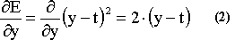
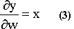
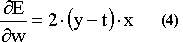
First we will consider the linear case, where the output of the network y equals the netinput a of the node.

What we are looking for is a way to update the value of the weight in order to make the error of the output minimum. One expression to calculate the error of such a network is the following: E=(y-t)². This is quite a nice expression because it has some useful properties. 1) The bigger the difference between our output and the target, the bigger the error E. 2) Due to squaring, it will make no difference if our output is, for example, 10 units bigger than our target or 10 units smaller than our target. These mistakes are equivalent; they are equally error. 3) It is easy to handle mathematically.

The error E depends on the output y which depends on the weights since y=a=w^.x. Therefore the error is a function of the weights. We want to modify the weights in a way to decrease the error. From what we discussed before, differentiation is the appropriate "tool" that gives us information about how a function changes when we make a small change to one of its variables. We have to differentiate the error with respect to the weight. This calculation will eventually lead us to the following linear delta rule:

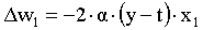
For more than one input in our single unit, e.g. x₁, x₂, ..., x_n and their corresponding weights w₁, w₂,..., w_n we will use one equation for each weight.

Delta rule for the first weight:

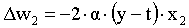
Delta rule for the second weight:

etc. We prefer to write these expressions in a general way :

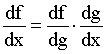
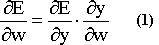
where i is an index, taking values from 1, 2, 3 etc. depending on the number of our inputs.

If you are interested in how the linear delta rule has been derived read the following section, otherwise go to exercise 6.

Such a calculation will be much more easier if we use the chain rule.

The combination of these three equations (1,2,3) will lead to:

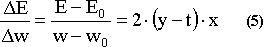
If you recall the definition of the differentiation, for small changes of the weigh, we can write equation 4 in the following form:

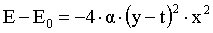
Assume that the weight of our network has the value w₀ and the error due to this weight is E₀. We wish to change the weight w₀ to a new value w, which will be close to w₀ but will result an error E smaller than the error E₀. We would like to ensure that E<E₀, which means E-E₀<0. Rewriting the previous equation as: E-E₀=2(y-t)^.x^.(w-w₀) we want to pick up a value for (w-w₀) which will lead to a negative second part of the equality, regardless of the values of y,t and x. Take:

where is a positive real number. In this case:

which will be negative at any rate since a is positive and any number squared is also positive. Choosing the new w according to equation (6) we can be sure that the error will be decreased if we decide on a small value for , since the differentiation of a function is dealing with input variable values (in our case w) that are very close to each other. We have then developed a linear learning delta rule (eq 6).

6. In exercise 12 of the previous lab you designed a simple neural network that implements the logical AND function. However you had used predefined values for the weights. Now you can redesign the same network with a training process. Given the input and the target, your network should compute the appropriate values for the weights. A rough description of the process follows:

   i) Give an initial value to the weights. Usually we randomize the weight values using a random number generator. You may use Matlab function rand.

   ii) Calculate the output of the network, using the first of the input sets (commonly named training data), calculate the error and update the weights according the linear learning rule. Then go to the second set and repeat the same process. When you are done with each one of the input sets, you have completed an epoch. At the end of the epoch you have to calculate the average error of all input sets. Repeat ii) for a specific number of epochs. Remember to set average error to zero at the start of each epoch, since it is meant to count the average error of one particular epoch.

Non-Linear delta rule.

Quite often though, as we mentioned in lab 1, the activation (netinput) is not equal with the network output, but it is used as input to a function whose output is the network output. In many cases this function is the sigmoid function. In such cases we can develop a non-linear learning rule, similar to the linear case.

7. Plot the sigmoid function:

   

   Type:
   >> a=linspace(-10,10,50);
   >> y=1./(1+exp(-a));
   >> plot(a,y)

   On the same graph plot the first derivative of the sigmoid function. It can be proved that the first derivative y´=y.(1-y).

   Type:
   >> hold on
   >> plot(a,y.*(1-y));
   

The learning delta rule that can be developed when the activation of the neural unit passes through a sigmoid function is:

Note that we may omit the 2 from both learning rules by choosing a suitable .