 (Size halved to reduce data volume)
This teach file introduces active contour models of shape, or snakes.
Please read the introduction giving general information about the nature of this document.
You must have read and understood TEACH VISION1. It will be helpful to have looked at subsequent teach files.
First, load these libraries to avoid having to do it as you go along,
    uses popvision          ;;; search vision libraries
    uses sunrasterfile      ;;; for reading image files
    uses float_byte         ;;; type conversion
    uses convolve_gauss_2d  ;;; smoothing and smoothed centre-surround
    uses float_arrayprocs   ;;; array arithmetic
    uses canny              ;;; for edge detection
    uses ellipse_hough      ;;; for ellipse finding
    uses squared_gradients  ;;; for image gradients
    uses snakes             ;;; for snakes
read in an image,
    vars image;
    sunrasterfile(popvision_data dir_>< 'clock.ras') -> image;
make sure we are working in degrees and have enough memory
    false -> popradians;
    max(popmemlim, 15e5) -> popmemlim;
We will also need a smoothed version of the image:
    vars simage;
    convolve_gauss_2d(image, 3.0, false) -> simage;
In computer vision, recognising objects often depends on identifying particular shapes in an image. This is a difficult task and a central problem in vision. The area of shape representation is concerned with finding ways of describing shape that are sufficiently general to be useful for a range of objects, whilst at the same time allowing their computation from image data, and facilitating comparisons of similar shapes. Both 2-D and 3-D shapes need to be modelled, and a very wide range of ideas can be found in the literature. One of the best known of 3-D representations is Marr's hierarchical approach based on generalised cylinders, described in his book Vision. This teach file is concerned with the slightly simpler area of 2-D shape, and one particular kind of representation that can be relatively easily matched to image structure. It also illustrates the very general mechanism of optimisation as a way of finding structure.
Look at the image read in above:
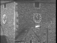
rci_show(image) -> rc_window;
(Size halved to reduce data volume)
(The assignment to rc_window will allow graphics operations on the window later.)
Suppose we are interested in the outlines of the clockfaces. We might start by looking to see whether image edges will help - so we might try a Canny-type edge detector (see TEACH VISION3):
    vars edges;
    canny(image, 2, 3, 10) -> ( , , edges);
    rci_show(float_threshold(0, 1, 1, edges, false)) -> ;
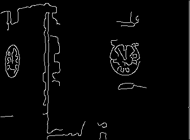
As it happens, with these parameters, there is a simple contour round the left clockface, but the contour of the right clockface is rather broken up. In addition, bits and pieces of other structure inevitably show up in the edge map. Clearly, using an edge detector alone, however good it is, will not separate the clockfaces from other structure in the image. We need to bring more prior knowledge to bear on the problem.
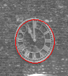
The edge detector is entirely local and makes no assumptions about the shape that is of interest. Going to the other extreme, suppose we know in advance the exact shapes of the clockfaces' images. They are elliptical and elongated along the Y direction. The one on the right has a extent of about 62 pixels in Y and about 56 pixels in X. With this much prior knowledge, it is easy to find it in the image. We can, for instance, use a simple 2-parameter Hough transform (see TEACH VISION4 and HELP * ellipse_hough) and exploit the edges we have detected, thus:
    vars xc, yc;
    ellipse_hough(edges, 31, 28, 90) -> (xc, yc);
(The 31 and 28 arguments are half the ellipse dimensions mentioned above and the 90 is the angle between the long-axis of the ellipse and the X-axis. We are assuming that somehow these are known in advance.)
Using the mouse, move or destroy the edge image window so that it does not obscure the original image. Then plot the ellipse we have found with
    rci_show_setcoords(image);
    'red' -> rc_window("foreground");
    appellipse_rim(xc, yc, 31, 28, 90, image, rci_drawpoint);
 (Image cropped to reduce data volume)
(See HELP * appellipse for details.)
The left clockface is similar but is more foreshortened so only has an extent of about 26 pixels in X. We can therefore find it with
    ellipse_hough(edges, 31, 13, 90) -> (xc, yc);
    appellipse_rim(xc, yc, 31, 13, 90, image, rci_drawpoint);
 (Image cropped to reduce data volume)
We have found the clockfaces by using extremely exact 2-D models of their images - ellipses with known dimensions and orientations. It is unreasonable to expect that such detailed information will normally be known in advance. We would like to weaken the assumptions.
One way to do this might be to use a more general Hough transform, or some other method, that can detect any ellipse, and this might well be appropriate in some applications. However, we might want to weaken the conditions further, and look for a shape in the image that is smooth and forms a closed contour, but which is not necessarily elliptical.
Active contour models, or snakes, allow us to set up such general conditions, and find image structures that satisfy the conditions.
To illustrate this, suppose we know that there is a clockface in the rectangular region of the image with opposite corners at X = 200, Y = 70 and X = 310, Y = 170. We can set up a snake to start on this rectangle with the following code (ignore the details for now):
    vars snake;
    coords_to_snake(200,70, 310,70, 310,160, 200,160, 4) -> snake;
    interp_snake(snake, false, 10) -> snake;
and see it with
    rci_show(image, rc_window) -> rc_window;    ;;; get rid of ellipses
    display_snake(snake, image, 'red', 'red', rc_window) -> rc_window;
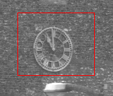 (Image cropped to reduce data volume)
Now we can tell the snake to shrink, to try to form a smooth contour, and to avoid going onto brighter parts of the image.
    evolve_snake(simage, snake, 0.4, 0, -0.08, 'green', 'green',
        0.1, 150, image, rc_window) -> snake;
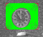 (Image cropped to reduce data volume)
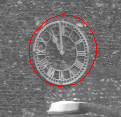
The final position of the snake is shown with
    rci_show(image, rc_window) -> rc_window;
    display_snake(snake, image, 'red', 'red', rc_window) -> rc_window;
 (Image cropped to reduce data volume)
The snake has converged on the contour of the outside of the clockface, distorted a little by the bright flint at 1 o'clock.
The remainder of this teach file is concerned with explaining how this kind of active contour model operates.
For this teach file, the snakes used have a very simple form. They consist of a set of control points, effectively connected by straight lines. Each control point has a position, given by (X, Y) coordinates in the image, and a snake is entirely specified by the number and coordinates of its control points. Adjustments to the snakes are made by moving the control points. The control points were not shown separately in the example above, for in future examples will be picked out in a different colour. All the snakes used here form closed loops in the image, though this is not necessarily true of snakes in general.
(If you are interested in data structures, you may like to know that the coordinates of a snake are held in two circular lists. In a normal Pop-11 list, the back of the last pair points to nil. In circular lists, the back of the "last" pair points to the "first" pair - which means that if you keep taking the tail, you end up back where you started after going through all the intermediate pairs. The implementation, unlike that of some of the popvision libraries, is entirely in relatively straightforward Pop-11 - as with all the libraries, you can look at the code, in this case by looking at LIB * SNAKES.)
One of the chief virtues of snake representations is that it is possible to specify a wide range of snake properties, through a function called the energy by analogy with physical systems. A program controlling a snake causes it to evolve so as to reduce its energy, so by specifying an appropriate energy function, we can make a snake that will evolve to have particular properties, such as smoothness.
The energy function for a snake is in two parts, the internal and external energies. Thus
    E       =   E         +  E
     snake       internal     external
The internal energy is the part that depends on intrinsic properties of the snake, such as its length or curvature. The external energy depends on factors such as image structure, and particular constraints the user has imposed. Some examples of each follow.
The physical analogy can be extended, and the motion of the snake can be regarded as being due to simulated forces acting on it. Just as the forces on physical systems always make them move so as to reduce their energy, so the simulated forces on a snake are arranged to make it reduce its total energy. To design a snake with specified properties, it is normal to work out a suitable energy function and then calculate the forces needed to reduce it.
A particularly simple energy function is the "elastic band" internal energy that was used to make the snake shrink in the example above. This is examined next.
If we want the snake to shrink, we need to define an energy that increases with its length. An energy proportional to the total length seems the obvious choice, but in fact there is a better one.
The snake will be better behaved if the control points are equally spaced round it, rather than being bunched up, and we can arrange for this by making the contribution to the energy extra large for two control points that are further apart than average. A convenient form for an energy function with this property is the sum of the squares of the distances between adjacent control points. Taking the squares increases the contribution of unusually widely spaced control points even faster than if the energy was just the total length.
This is, roughly, the energy of a physical snake in which the control points are joined together by springs obeying Hooke's law. (Roughly, because the springs would have to shrink to zero length when released, and most real springs have a finite resting length.) It's useful to multiply the sum by an adjustable constant. The constant corresponds to the strength of the springs.
The energy can be written as
                      N                                      2
 E          =   K1 * SUM  (distance between control point i)
  elastic            i=1  (     and control point i-1      )
where N is the number of control points and K1 is an arbitrary constant that can be set to whatever value suits us. The symbol i is the index of a control point. Because the snake is a loop, we interpret control point 0 as being the same as control point N.
The form
                        N
                       SUM
                       i=1
means that for each value of i from 1 to N, we work out the value of the expression that follows, and add up the results. A mathematical formula with SUM in it translates into a for loop in Pop-11 code (for i from 1 to N do ...), where some variable, initially given the value zero, has the value of the expression added on to it at each iteration. The symbol written here as SUM is actually printed as the capital greek letter sigma, which looks a bit like this:
                        ---
                        \
                        /
                        ---
The square of the distance between control point i and control point i-1 is given by Pythagoras' formula
               2                  2
    (x  - x   )    +   (y  - y   )
      i    i-1           i    i-1
where
       (x , y )
         i   i
are the coordinates of control point i.
How does this energy translate into a force on the control points? To work this out, it is necessary to deduce a formula giving the energy changes for an arbitrary motion of the control points, and hence to find the motion that reduces the energy most. The tool that is needed for this is the differential calculus. If you understand calculus, you may be able to verify the next equation, but if not, you can take it on trust.
The elastic force on the i'th control point has components in the X and Y directions given by
    F              =   2 * K1 * ( (x   - x )  +  (x   - x ) )
     elastic_X,i                    i-1   i        i+1   i


    F              =   2 * K1 * ( (y   - y )  +  (y   - y ) )
     elastic_Y,i                    i-1   i        i+1   i
Look at the first part of the X expression. If x(i) (using brackets instead of subscripts) is less than x(i-1), then the X component of this part of the force is positive. If x(i) is greater than its x(i-1), the contribution is negative. That is, the i'th control point is pulled along the X axis towards the i-1'th point. The second half of the same expression says the point is also pulled towards the i+1'th point. The same thing occurs along Y. In short, the control point is simply pulled towards its two nearest neighbours.
Geometrically, the force is towards the average position of the neighbours. In this figure, control points are marked as o, and the * is supposed to be half way between the i-1 and i+1 control points:
        |            _
        |            /|
    i-1 o           /
         \         / Elastic force on i along this line
          \       /
  snake -> \     * <- half way between i-1 and i+1 points
            \   /
             \ /
              o-----------o---------
              i          i+1
It should be clear that such a force applied to every control point will pull the snake inwards and will pull the control points into line with one another, smoothing the snake. It may seem obvious that this is what is wanted, and that consideration of the energy was superfluous; indeed for simple properies one might just define a suitable force straight away. For more complex properties, though, it is much easier to start with an energy that expresses the quality required, and then work out the force expressions from it.
Now we know what force acts on each control point, we have to use it to adjust the position of the snake.
Once we have an expression for the force, we can implement the dynamics of the snake simply. At each time step, we simply move each control point by an amount proportional to the force acting on it. In the physical analogy, this is like making a light snake move through a viscous fluid - it should dissipate its energy without oscillating.
The updating equation is therefore
         x    +   K2 * F            ->   x
          i             elastic_X,i       i
and the same thing for Y. K2 is another user-defined constant, which says how fast the point can move for a given force. In practice, we calculate the new coordinates for all the points before updating any of them - i.e. we use the old value of x(i), not the new one, to find the shift in x(i+1).
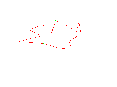
Here is a snake obeying this equation. First, blank the window:
rci_show(boundslist(image), rc_window) -> rc_window;
and set up and display a snake
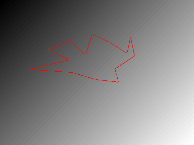
    vars snake0;
    coords_to_snake(
        139,82,170,109,183,68,217,84,252,106,259,74,267,111,228,
        137,235,163,190,158,143,144,60,138,138,119,96,99, 14) -> snake0;
    snake0 -> snake;
    display_snake(snake, image, 'red', 'green', rc_window) -> rc_window;
Now we cause it to take one step to reduce the elastic energy. The procedure has an argument alpha which is equal to 2 * K1 * K2 to control how much the points move. This should normally be much less than 1. We here set it to 0.1. The other arguments just say that there is no other force on the snake.
    adjust_snake(snake, 0.1, 0, 0, snake_nullforce) -> (snake, );
    display_snake(snake, image, 'red', 'green', rc_window) -> rc_window;
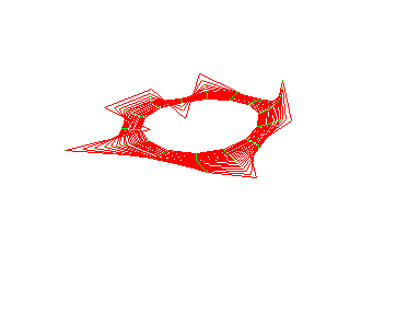
(After executing the code 20 times)
If you keep executing the two lines above, you will see that the elastic force rapidly pulls the snake into a smooth oval, which keeps contracting. The most outlying points get pulled in fastest. One or two points start moving outwards because they are pulled into line with their neighbours before the overall contraction gets to them. After a few iterations you can also see the trajectories of the control points, which move to be equidistant from each other.
What we have done is to simulate a physical system in order to give a computational structure the property we want.
It is sometimes useful for a snake to behave like a thin metal strip rather than, or as well as, like an elastic band. That is, it should try to be a smooth curve or straight line, but should not contract. This can easily be done by defining the right energy function.
Details will not be given here, but the energy function in this case is the sum of the squared curvatures of the snake measured at the control points. The sharper the angle made by the nearest neighbours at the control point, the bigger the curvature. In practice, a simple approximation to the curvature is used. This energy translates into forces at each control point that depend on its 4 nearest neighbours, not just the nearest two as for the elastic force, and which tend to straighten out the snake. (You can see the exact form of the force by looking at the code for adjust_snake in LIB * SNAKES.) These forces are hard to work out directly, but easy to obtain from the energy.
To demonstrate the effect, we use the same code but set the constant beta, which controls the size of the bending energy's effect, to 0.05, whilst alpha is zero to switch off the elastic force. First, go back to the start:
    rci_show(boundslist(image), rc_window) -> rc_window;
    snake0 -> snake;            ;;; initialise snake
    display_snake(snake, image, 'red', 'green', rc_window) -> rc_window;
and then iterate these two lines
    adjust_snake(snake, 0, 0.05, 0, snake_nullforce) -> (snake, );
    display_snake(snake, image, 'red', 'green', rc_window) -> rc_window;
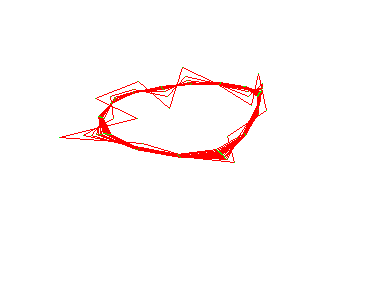
(After executing the code 20 times)
In fact, because the simulation is an approximation, the snake will still tend to shrink slightly, but the dominant effect is now smoothing rather than shrinkage.
In the model implemented here, the internal energy is just the sum of the elastic and bending energies, their proportions controlled by the alpha and beta constants.
Now we turn to the external forces on the snake. These determine its relationship to the image. Suppose we want a snake to latch on to bright structures in the image. Then the obvious energy function is minus the sum of the grey levels of the pixels the snake is on top of. Reducing this energy function (i.e. making it more negative) will move the snake towards brighter parts of the image.
In this implementation, the energy is actually only calculated for the pixels which lie under control points, not under the straight lines between them. Thus the image energy is
                            N
        E       =   - K3 * SUM  image(x , y )
         image             i=1         i   i
where image(x, y) is the grey level of the pixel at (x, y) in the image. K3 is just another user-selected constant. The force that this produces again turns out to have a rather simple approximation:
 F           =   K3/2  * ( image(x + 1, y ) - image(x - 1, y ) )
  image_X,i                       i      i           i      i


 F           =   K3/2  * ( image(x , y + 1) - image(x , y - 1) )
  image_Y,i                       i    i             i    i
That is, if the pixel in the direction of increasing X is brighter than the pixel in the direction of decreasing X, then the control point is pulled in the positive X direction, and likewise for Y. In short, the force on the control point is in the direction of the grey-level gradient.
We can demonstrate this most clearly by using an image which has the same gradient everywhere. This generates and displays an array with such a property:
    vars grad_image;
    newsfloatarray(boundslist(image), nonop +) -> grad_image;
    rci_show(grad_image, rc_window) -> rc_window;
and we again set up our snake:
    snake0 -> snake;            ;;; initialise snake
    display_snake(snake, image, 'red', 'green', rc_window) -> rc_window;
Now we switch all the internal forces to zero, but supply an external force which corresponds to the above formula, using a closure of snake_imforce. The rate of motion due to the external force is given by a control constant called gamma, which we set to 0.5. Now iterate this code:
    adjust_snake(snake, 0, 0, 0.5, snake_imforce(%grad_image%))
        -> (snake, );
    display_snake(snake, grad_image, 'red', 'green', rc_window)
        -> rc_window;
finishing up with
    display_snake(snake, grad_image, 'blue', 'green', rc_window)
        -> rc_window;
(After executing the code 20 times)
The snake stays the same shape but wanders in the direction of the brighter part of the image.
If you make gamma negative, the snake will go the opposite way.
Many real images have a lot of small-scale noise or structure, which will disrupt the progress of the snake by applying large, randomly varying forces, if we just use the force formulae as given above. Also, it is clear that with these formulae, the snake only "sees" image structure that is within 1 pixel of the control points. To avoid the effects of very local structure, and to give the snake more of a chance to find structures that are not right next to it, more useful snakes use a more sophisticated estimate of the grey-level gradient, which averages over more pixels. This is equivalent to using the simple formulae on a smoothed version of the image. In this teach file, snakes with simple image forces are used with a smoothed image (simage, which was set up at the start) instead of using a more complex formula for the image forces.
A snake being used for image analysis attempts to minimise its total energy, which is the sum of the internal and external energies. When energies are added their associated forces add too. In the first snake example in this file, finding the clockface, the snake had an elastic energy and an image energy, but no bending energy. The parameter gamma was negative, so the image energy drove the snake towards darker parts of the image. The snake contracted under the elastic force until this was balanced everywhere by the image force, and it came to rest shrink-wrapped round the clockface.
To explore this balance of forces, it is convenient to be able to initialise a snake on any part of the image.
Snakes have to started off somewhere in the image. So far we have ignored this point, but in the seminal paper on snakes (Kass, M., A. Witkin & D. Terzopoulos, 'Snakes: Active contour models', in Proceedings, First International Conference on Computer Vision, London, England, pp 259-268, IEEE, Piscataway, NJ, 1987), snakes are regarded as a "power assist" for a human operator needing to measure structures in images. The operator would point the snake at, say, particular cells in a histological image, or at a road in a satellite image, and the snake would lock on to it and provide an accurate measure of its shape.
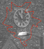
To start a snake on the clock image by pointing, execute the following line of code. Then move the cursor into the image window, and click the left-hand mouse button at the position you want the first control point to be. Moving the cursor round the outline of the snake, keep clicking the left-hand button to fix the position of each corner. When you are almost back to the starting point, click the right-hand button.
    get_snake(image, false, 10, 'red', 'yellow', rc_window)
        -> (snake, rc_window);
 (Image cropped to reduce data volume)
Make sure the snake does not get close to the edge of the image. You might try putting a snake round the left clockface, or round the right clockface and the street light, or round all three. The snake will have control points separated by about 10 pixels, regardless of how often you clicked the mouse button.
Having initialised the snake, it might be worth saving it so that you can go back to the same starting point, with
snake -> snake0;
Now you can evolve the snake, either a step at a time as above, or by executing evolve_snake with suitable parameters:
    vars alpha = 0.2;       ;;; elastic forces
    vars beta = 0.05;       ;;; bending forces
    vars gamma = -0.1;      ;;; image forces
    evolve_snake(simage, snake, alpha, beta, gamma, 'green', 'green',
        0.05, 100, image, rc_window) -> snake;
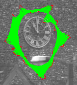 (Image cropped to reduce data volume)
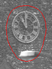 Final position (Image cropped to reduce data volume)
If you get an "invalid array subscript" mishap, you probably made the snake too close to the edge of the image. Rerun get_snake and try again. You can repeat the call to evolve_snake to make it continue from where it stopped if a balance has not been reached after 100 iterations. See HELP * SNAKES for full details of the arguments, and note that although image is displayed in the window, the procedure actually refers to simage to calculate the image forces.
To restart from the same initial snake, do
    rci_show(image, rc_window) -> rc_window;
    snake0 -> snake;
before going back to evolve_snake.
You may well need to adjust the values of alpha, beta and gamma to get the behaviour you want. You should be able to guess what effect changing their relative values will have. Be careful not to make them too large - beta particularly should be less than 0.1 - or the snake will become unstable and the control points will move wildly until they go outside the image, causing a mishap.
So far, the snake has had an image energy with the effect of repelling it from brighter regions of the image. It is not difficult to change this, for example to make the snake try to find edges. Then, the energy would decrease if the snake was lying on a region of high image gradient. (See TEACH VISION3 for a description of image gradient.)
It is easiest to demonstrate this in the present setup by producing an array of image gradients, and making the snake operate on this, just as the snake has been working with a smoothed version of the clock image. We will have a change of image for this:
    sunrasterfile(popvision_data dir_>< 'butterfly.ras') -> image;
    rci_show(image, rc_window) -> rc_window;
(Image cropped and snake outline included to reduce data volume)
Now generate the squared smoothed gradient (this is a little like the raw material for *canny, except without the peak detection). This will take a little time. We then display the result.
    squared_gradients(image, 6.0, false, false) -> simage;
    rci_cmap("sqrt");           ;;; make weak edges more visible
    rci_show(simage) -> ;
    rci_cmap("linear");         ;;; back to normal display grey-levels
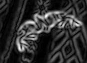 (Size halved to reduce data volume)
The second argument to squared_gradients, 6.0, is a smoothing constant (sigma) which is used to blur the image for the same reasons that we smoothed the clock image. Move the gradient image window if necessary to make the original image visible.
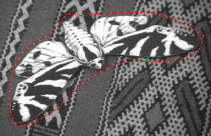
Here is a snake that starts out close to the butterfly's outline
    coords_to_snake(
        100,122,123,105,148,89,163,66,191,69,220,66,249,64,279,64,308,
        71,335,82,360,98,352,122,324,133,295,136,265,135,236,137,
        210,151,186,166,166,186,146,207,120,221,91,229,82,206,81,
        176,86,147,  25) -> snake;
    interp_snake(snake, false, 10) -> snake;
    display_snake(snake, image, 'red', 'yellow', rc_window) ->
        rc_window;
(Image cropped to reduce data volume)
This code evolves it with the image energy coming from the gradients:
    evolve_snake(simage, snake, 0.1, 0, 0.05, 'blue', 'green',
        0.2, 150, image, rc_window) -> snake;
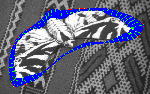
(Image cropped to reduce data volume)
At the back of the butterfly, the image energy dominates and the snake is pulled in to fit quite closely onto its contour. Note how it neatly interpolates across gaps in the white outline at the back of the wings. At the front, however, there are weaker edges, and the elastic energy dominates, so that the snake remains stretched tight in front of the butterfly's nose. The final position is more visible with
    rci_show(image, rc_window) -> rc_window;
    display_snake(snake, image, 'red', 'green', rc_window) -> rc_window;
(Image omitted to reduce data volue - final position is innermost contour in previous image.)
You may wish to experiment with other snakes initialised using the mouse, and with changing the parameters.
Optimisation in this context means using mathematical techniques to find the maximum or minimum of a function, and is not to be confused with optimising a program, which usually just means trying to make it run faster. The function to be minimised here is the total snake energy.
Working out the forces and using them to move the control points is just one kind of optimisation technique. This particular method is known as gradient descent, and is used in many other contexts, such as the backpropagation algorithm for training feedforward neural nets. It is closely related to hill-climbing search methods.
Although very simple to implement, gradient descent is actually rather crude, and requires small movements at each time step to work properly. If you try making alpha or beta too large in the examples above, you will see what this means.
Better techniques are possible, particularly in connection with the internal energy. Because the internal energy function depends only on the control point coordinates, and not on the image, it is possible to calculate directly the configuration of the snake that will cause the internal forces to balance a given set of external forces. This means that the algorithm can become:
 until enough iterations have been done or balance has been reached
     calculate the external forces for the current position
     move so that the internal forces balance these external forces
 enduntil
This allows bigger steps to be taken, and is more efficient overall despite the extra computation involved in the second stage. The calculation of the new position involves numerical inversion of a matrix, but the matrix has a special structure that makes this not too expensive. The search technique called dynamic programming has also been applied to speeding up snake evolution in a similar way.
The snakes used in the demonstrations in this teach file have fairly simple properties. It is possible to give snakes a much wider variety of properties to make them applicable to a range of problems. For example:
The snakes demonstrated here have all been initialised by hand. For real computer vision, it is necessary to have some automatic way of starting the snakes. Again, there are various possibilities.
Given enough computing power, it is possible to start off many snakes at random, and see which ones find structures they like. The others can be killed off.
Conventional techniques can be used to find structures to start the snakes. For instance, in image sequences, differencing (see VISION6) might provide regions of interest round which snakes can be put. In other cases, a Hough transform or other recognition techniques can provide a starting point. Groups of line segments or unusual texture, colour or intensity patches might be used.
Snakes are computationally cheap compared to many other image processing operations, so can be added on to other systems to improve their final performance.
You should now:
Here are links to:
Copyright University of Sussex 1995. All rights reserved.