This teach file continues with the theme of convolution, introducing biological models and practical edge detection methods which rely on convolution with Gaussian masks. The effects of image analysis at different scales are also illustrated.
Please read the introduction giving general information about the nature of this document.
You should have read TEACH VISION1 and VISION2.
Load the necessary libraries and get hold of an image now:
    uses popvision          ;;; search vision libraries
    uses rci_show           ;;; image display utility
    uses arrayfile          ;;; array storage utility
    uses float_byte         ;;; type conversion utility
    uses float_arrayprocs   ;;; array arithmetic library
    uses convolve_gauss_2d  ;;; Gaussian convolution program
    uses rc_graphplot       ;;; graph display utility
    uses canny              ;;; Canny edge detection
vars image;
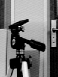
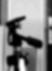
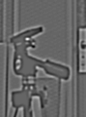
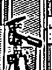
arrayfile(popvision_data dir_>< 'stereo1.pic') -> image;
float_byte(image, false, false, 0, 255) -> image;
The Gaussian convolution mask is a circularly symmetrical (or isotropic) mask, such that any cross-section through its centre yields a weight profile that has the form of a Gaussian or normal curve. The mathematical formula is in all statistics text books, and almost all computer vision books. A Pop-11 procedure which implements the formula to generate Gaussian weights looks like this:
    define gauss_weight(r, sigma) -> g;
        lvars r, sigma, g;
        exp( -(r**2) / (2 * sigma**2) ) -> g
    enddefine;
The r argument gives the distance (in pixels) from the centre of the mask, and sigma specifies the "width" of the mask. The procedure returns the weight for this distance and width parameter. We can see what the curve looks like by plotting the function with *RC_GRAPHPLOT:
    rc_new_window(400, 300, 500, 20, false);  ;;; make a new window
    rc_graphplot(-13, 1, 13, 'r', gauss_weight(% 5 %), 'G') -> ;
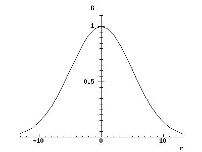
If the graph window appears in an inconvenient place on the screen, move and resize it with the mouse, then if necessary re-execute the call to rc_graphplot.
To draw the graph, sigma was set to 5 by creating a closure (see *CLOSURES) of gauss_weight. You can see that the curve drops to about 60% of its central value when r is equal to sigma - this is what is meant by by saying that sigma sets its width. Try changing sigma to see the effect.
The mathematical Gaussian function does not fall to zero for any finite value of r - the "tails" of the curve go on forever. For a practical mask, it is necessary to truncate the function when the weights have become small enough to be insignificant, to keep the mask to a reasonable size. As you can see from the graph, the values are pretty small when r is plus or minus 13 for sigma = 5. An efficient library procedure to generate arrays containing Gaussian weights is gaussmask. This has a sensible criterion for truncation built in (see HELP *GAUSSMASK), and it also normalises the weights - that is, it multiplies them by a constant so that the weights in the mask sum to 1, which avoids increasing or decreasing the average grey-level when the mask is used for smoothing. To get a 1-D Gaussian mask, execute:
    vars gmask, gsize, sigma;
    5 -> sigma;
    gaussmask(sigma) -> gmask;          ;;; calculate the weights
    gaussmask_limit(sigma) -> gsize;    ;;; get the mask size
The bounds of the mask array are given by [-gsize gsize]. If you plot the values in gmask with rc_graphplot (it will accept an array as an argument instead of a function) you will find the curve looks the same as the one we already have, though the actual values are smaller because of normalisation. A fast and simple way to print the values in the gmask array is:
    gmask =>                    ;;; print the boundslist
prints:
    ** <array [-13 13]>

    arrayvector(gmask) =>       ;;; see HELP *ARRAYS
prints:
    ** <sfloatvec 0.002735 0.00451 0.007144 0.010873 0.015899 0.022337 0.030152
        0.039105 0.048727 0.058337 0.067104 0.074161 0.078747 0.080338 0.078747
        0.074161 0.067104 0.058337 0.048727 0.039105 0.030152 0.022337 0.015899
        0.010873 0.007144 0.00451 0.002735>
but this method is only really useful for small 1-D arrays.
We can get a 2-D Gaussian mask by multiplying elements of the 1-D mask together. (This is because the 2-D Gaussian mask has a convenient property called separability; you would have to go back to the formula and do some algebra to demonstrate this, which we will not do here.) We can therefore generate a 2-D Gaussian mask with a little sleight-of-hand, using a procedure as initialiser for newarray:
    vars gmask_2d;
    newarray([% -gsize, gsize, -gsize, gsize %],
        procedure(x, y); lvars x, y;
            gmask(x) * gmask(y)
        endprocedure) -> gmask_2d;
We can now look at the 2-D gaussian mask with
    5 -> rci_show_scale;            ;;; expand the display size
    rci_show(gmask_2d) -> ;
    1 -> rci_show_scale;            ;;; reset the display size
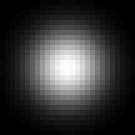
Of course, a digital mask like this is only an approximation to the mathematical Gaussian because it has been sampled on a discrete grid and truncated. However, it is good enough for practical use.
The Gaussian convolution mask is important both in theories of biological vision, such as Marr's, and in many computer vision systems. As a smoothing mask, it has optimal properties in a particular sense: it removes small-scale texture and noise as effectively as possible for a given spatial extent in the image.
To analyse this property fully requires a mathematical development that is beyond the scope of this course, and requires careful definition of terms like "spatial extent" used loosely above. One key idea, that is useful to know about even without the mathematics, is that of spatial frequency. High spatial frequencies correspond to small-scale structure; low frequencies to large scale structure. It is possible to decompose an image into its constituent spatial frequences, just as it is possible to decompose a sound wave into its constituent temporal frequencies (which we hear as different pitches). Spatial frequency analysis is used in some practical methods in image processing, and is an important psychophysical tool in investigations of biological vision.
Since small-scale texture contains a lot of grey-level variation at high spatial frequencies, the aim of a smoothing operation is to remove high spatial frequencies without distorting lower spatial frequencies. It turns out that because the Gaussian mask is itself smooth, it is particularly good at separating high and low spatial frequencies without using information from a larger area of the image than necessary.
We will use the procedure convolve_gauss_2d to try out Gaussian smoothing and demonstrate its efficacy. (This procedure is much more efficient than a general procedure like convolve_2d, because it makes use of the separability property to greatly reduce the amount of computation.)
It will be useful to have a test image to look at: we can generate one with a stripy pattern as follows
    vars testimage;
    newsfloatarray([1 100 1 100],        ;;; float array for efficiency
        procedure(x, y) -> value; lvars x, y, value = 0;
            if x mod 20 > 9 then
                20 -> value
            endif;
            if y mod 4 > 1 then
                20 + value -> value
            endif
        endprocedure) -> testimage;
    2 -> rci_show_scale;
    rci_show(testimage) -> ;
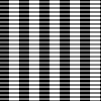
This gives an array with a high spatial frequency (i.e. fine) grid intersecting a low spatial frequency (i.e. coarse) grid. Now we examine the effect of Gaussian smoothing with sigma = 4.
rci_show(convolve_gauss_2d(testimage, 4)) -> ;
The fine stripes are effectively filtered out, leaving the broad ones. If we try the same thing with a uniform mask, it is impossible to do it as effectively - e.g. a 7 x 7 mask gives these results
    vars umask, usize;
    3 -> usize;         ;;; -3 to +3 gives a 7 x 7 mask
    newarray([% -usize, usize, -usize, usize %], 1.0/(usize**2)) -> umask;
    rci_show(convolve_2d(testimage, umask, false, false)) -> ;
Changing the size of the mask will not improve the results significantly. The reason is that the uniform mask has an abrupt cut-off at its boundaries, so as it passes over the thin stripes and their edges cross the mask boundary, sharp changes in the output values are inevitable. It is this sharp cut-off that the Gaussian mask avoids.
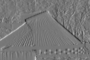
Now look at the effects of Gaussian smoothing on the real image.
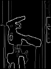
rci_show(image) -> ; ;;; no smooothing
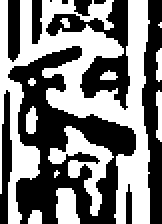
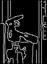
rci_show(convolve_gauss_2d(image, 1)) -> ; ;;; sigma = 1
rci_show(convolve_gauss_2d(image, 2)) -> ; ;;; sigma = 2
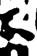
rci_show(convolve_gauss_2d(image, 4)) -> ; ;;; sigma = 4
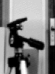
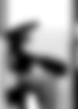
and note the increasing reduction in detail and fine texture, and the removal of all but the main shape in the final image.
It is reasonable to think of sigma as setting the scale at which we preserve information in the convolved image. Structure on a scale small compared with sigma will be removed, whilst structure on a larger scale is retained.
Many systems make use of structure at several scales, retaining multiple representations like the ones displayed by the code above. When the image has been smoothed, it is not necessary to retain as many pixels in the representation - one quarter of the pixels might be enough after smoothing with sigma = 2, for example. Smaller arrays are therefore used to hold the smoothed images, resulting in a data structure called a resolution pyramid.
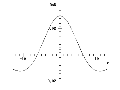
It has already been pointed out that a centre-surround mask can be used to locate grey-level boundaries in an image. It seems reasonable to combine the centre-surround operation with Gaussian smoothing to find the boundaries at different scales in the image. We could simply carry out the two operations one after the other, or generate a combined mask by convolving the Gaussian mask with the centre-surround mask, but it is usually more convenient to use the the difference of Gaussians mask, or DoG. The DoG is a good approximation to the combined centre-surround+Gaussian operator (which is also called the Laplacian of the Gaussian).
We can look at the form of the 1-D difference of Gaussians by generating two 1-D masks and subtracting one from the other. It turns out that the best approximation to the Laplacian occurs if the larger mask has a sigma about 1.6 times that of the smaller. This code will display the resulting curve (somewhat truncated):
    vars maskinner, maskouter, dogmask;
    gaussmask(5) -> maskinner;
    gaussmask(5 * 1.6) -> maskouter;
    gaussmask_limit(5) -> gsize;
    newarray([% -gsize, gsize %],
        procedure(r);
            maskinner(r) - maskouter(r)
        endprocedure) -> dogmask;

    rc_graphplot(-gsize, 1, gsize, 'r', dogmask, 'DoG') -> ;
(If the window containing the earlier graph has been iconified or is behind other windows, you will have to make it visible again.)
You can see that it has a smooth centre-surround structure, as expected. (We cannot use our earlier procedure gauss_weight to generate this curve, as it is important that the values in the positive and negative masks are normalised.)
The DoG is not separable. However, an efficient implementation is still possible by simply taking the difference between two Gaussian convolutions with different sigma values. We can look at the result of a DoG convolution with
rci_show(convolve_dog_2d(image, 1)) -> ;
where the second argument (1) is the sigma parameter for the inner part of the mask.
The raw output of the DoG operation does not yield any obvious simplification of the image. However, the significant features of the output of a centre-surround operator are the places at which positive and negative values are adjacent - its zero-crossings. For a full discussion of this, see Marr and other references in the bibliography in TEACH *VISION.
Note that the zero-crossings of any array that contains both positive and negative values can be found - the concept is not linked to any particular convolution operation. It is therefore wrong to talk about the zero-crossings of an image (as people quite often do); you need to refer to the zero-crossings of the output of the DoG operator, for example.
The most effective way to display the zero-crossings of a convolution operation is to threshold the output array. Thresholding is the operation of producing a binary image by assigning one value to all the pixels that exceed some limit (the threshold), and another value to all the others. (It is not usually very effective as a way of segmenting raw grey-level images, except in circumstances where the illumination and background can be carefully controlled.) We can apply it to visualising zero-crossings by setting the threshold to zero.
It is handy to have a small procedure to do the convolution, thresholding and display. The threshold procedure comes from *FLOAT_ARRAYPROCS:
    define showzeros(image, sigma);
        lvars image, sigma, newimage;
        convolve_dog_2d(image, sigma) -> newimage;
        ;;; Threshold so all values above 0 get set to 1, all others
        ;;; to -1. Re-use the array to reduce garbage collections.
        float_threshold(-1, 0, 1, newimage, newimage) -> newimage;
        rci_show(newimage) ->
    enddefine;
Now we can try it for a variety of scales. In the displays, the zero-crossings are, of course, the boundaries separating the black from the white regions - white shows the positive values and black the negative ones.
    showzeros(image, 1);
    showzeros(image, 2);
    showzeros(image, 4);
You can see how the positions of edges are accurately represented in the small-scale output, which also includes a lot of detailed texture, whilst the large-scale output retains the main features, but has only approximate positions for the edges.
Marr proposed that zero-crossings at different scales are combined by biological visual systems to obtain evidence for significant image boundaries. Whether this is so is open to doubt, but it is clear that processes analogous to DoG convolutions do operate in the early stages of biological vision. The results of such operations must therefore be an efficient way to code image structure, since retinal mechanisms have evolved to transmit this particular kind of information along the optic nerve. This makes sense: raw grey-levels, for example, contain a great deal of redundant information about the overall brightnesses of surfaces, whereas the DoG outputs sacrifice this to allow more information to be carried about texture and boundaries.
In practical computer vision, the DoG filter tends not to be used for edge detection. However, it has proved valuable in other ways - for example, a fast stereo-matching algorithm by Nishihara (to be discussed later) uses thresholded DoG convolutions to generate image regions to match. Furthermore, the idea of using zero-crossings for different values of sigma has been generalised into the important idea of scale space analysis.
We will leave the DoG at this point and turn to a popular edge-detector used in computer vision, but first it is necessary to say what is meant by the local grey-level gradient of an image.
The outputs of the X and Y differencing masks
                                      ------
              -----------             | -1 |
              | -1 | +1 |     and     |----|
              -----------             | +1 |
                                      ------
are often termed the X and Y grey-level gradients. If you imagine a surface above the image, whose height is proportional to the grey-level at each point, then it should be clear that what these operators give are measures of the slope, or gradient, of the surface if you move along the X and Y directions respectively. These measures can be combined to give the total gradient or gradient magnitude, which is how much the surface slopes in the direction which goes most steeply downhill. If the Y gradient is zero, for example, then the total gradient is just equal to the X gradient, but if the surface slopes in both the X and Y directions then we need to combine the two values.
The correct formula is, in fact, just that of Pythagoras:
                    2                 2               2
    (total gradient)   =  (X gradient)  + (Y gradient)
We can display the total gradient for our image:
    vars maskx, masky, imagex, imagey;
    newarray([0 1 0 1], 0) -> maskx;    ;;; for X differences
    -1 -> maskx(1, 0);
     1 -> maskx(0, 0);
    newarray([0 1 0 1], 0) -> masky;    ;;; for Y differences
    -1 -> masky(0, 1);
     1 -> masky(0, 0);
    convolve_2d(image, maskx, false, false) -> imagex;
    convolve_2d(image, masky, false, false) -> imagey;

    rci_show(float_arrayhypot(imagex, imagey, false)) -> ;
(We use 2 x 2 masks containing some zeros to make the X and Y gradient arrays come out the same size. For a practical program one would do something more efficient. The routine float_arrayhypot (from *FLOAT_ARRAYPROCS) takes its name from the fact that the Pythagorean formula calculates the hypotenuse of a triangle. It uses the C library routine hypot - see MAN *HYPOT.)
You can see how regions stand out where the grey-level changes most rapidly. It is also possible to calculate the gradient direction at each point in the image - i.e. the direction in the image for which the gradient changes most rapidly. For this you would use the C procedure atan2 or the Pop-11 procedure arctan2 applied to the X and Y gradients.
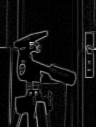
Although the DoG is not the basis for most edge detectors in computer vision, the idea of combining Gaussian smoothing with simple local operators certainly is. One of the more successful kinds of edge detector is based on ideas published by Canny (see Readings in Computer Vision, listed in the bibliography in TEACH *VISION, p. 184). This combines Gaussian smoothing with the simple horizontal and vertical difference operators. The results are then combined as above to give the total smoothed gradient at each pixel. Positions where the gradient is a local maximum along gradient direction are then found, and then a thresholding operation is used to find those lines where the gradient is above some limit. (Actually the thresholding is more complicated, but that is the basic idea.) For more details of the local implementation, see HELP *CANNY.
Canny's method can be applied to the usual image:
    vars edges;
    vars sigma = 1;         ;;; smoothing
    vars t1 = 5, t2 = 10;   ;;; hysteresis thresholds
    canny(image, sigma, t1, t2) -> (imagex, imagey, edges);
    rci_show(edges) -> ;
Here sigma is, as usual, the scale parameter for Gaussian smoothing, whilst t1 and t2 are thresholds used for deciding which parts of the edges to keep. In the display, the brightest edges are those with the strongest associated grey-level gradient. The other results returned by canny, imagex and imagey, are the smoothed X and Y gradients, which you can display for comparison with the unsmoothed versions we have looked at previously.
You could look at the Canny edges produced with different values of sigma, as we did for the DoG zero-crossings.
We can throw away the gradient strength information and make a binary array which records only the positions of edge pixels with:
    vars bin_edges;
    float_threshold(0, t1/2, 1, edges, false) -> bin_edges;
    rci_show(bin_edges) -> ;
This edge map often forms the basis for subsequent processing. For example, simple shapes like straight lines and ellipses can be found, particularly in the images of industrial objects to which computer vision is likely to be applied. These can be used to build up a geometrical description of the image at a higher level of abstraction. Alternatively, in model-based vision, the expected appearance of a model is often matched against the edge map.
You should now:
Here are links to:
Copyright University of Sussex 1994. All rights reserved.