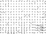
 (After 1 iteration)
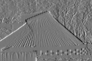
This teach file introduces the use of motion information in computer vision.
Please read the introduction giving general information about the nature of this document.
You need to have read and understood TEACH VISION1. It will be helpful to have looked at VISION2, VISION3 and VISION5.
Before proceeding, execute the following chunk of code to avoid having to load the libraries later.
    uses popvision          ;;; search vision libraries
    uses sunrasterfile      ;;; for reading image files
    uses filesequence       ;;; for reading image sequences
    uses float_byte         ;;; type conversion
    uses float_arrayprocs   ;;; array arithmetic
    uses first_order_flow   ;;; for flow pictures
    uses display_flow       ;;; for flow pictures
    uses horn_schunck       ;;; for optic flow measurements
    uses solve_dilation     ;;; for optic flow interpretation
As usual, the code in this teach file is designed to be run in the order in which it appears.
In stereoscopic vision (see TEACH VISION5), viewing a scene from more than one viewpoint simultaneously provides valuable information about 3-D structure. Moving the camera produces successive changes in viewpoint that can also yield this kind of information, but the changing image produced by movement, either of the camera or of objects in the environment, can also be used to provide direct predictive information useful in the control of action. In addition, motion can help with segmentation of the image into meaningful regions, and we begin with this application in the next section.
In practical computer vision, motion analysis requires the storage and manipulation of image sequences rather than single images. Image sequences can be stored in memory as lists of arrays, vectors of arrays or 3-D arrays, and on disc as single files or as files with sequential numbering. Each image in a sequence is often called a frame, and the time which elapsed between each frame being digitised the frame interval. The inverse of the frame interval, that is, the number of frames per second, is the frame rate. For systems based on the European TV standard, the maximum frame rate is usually 25 frames/second, though lower rates are often employed.
For many real applications such as robot control, the ideal is to process each frame as it arrives (in real time or online), but as this is likely to need specialised hardware, it is common for research purposes to store the images and process them at a lower rate, offline.
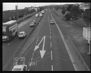
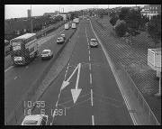
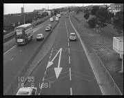
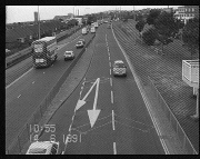
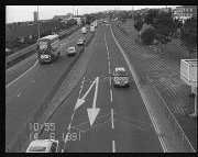
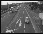
A special case of motion analysis is when the camera is actually static with respect to its environment, but other objects are moving. In practice, this is often the case for surveillance applications such as road traffic monitoring. A sequence of images captured under these conditions can be read from disc and displayed with:
    vars fname = popvision_data dir_>< 'shoreham';
    vars images = filesin(sunrasterfile, fname, 2, '.ras', 1, 1, 10);
    0 ->> rci_show_x -> rci_show_y; ;;; start display at top left
    40 ->> rci_show_xshift -> rci_show_yshift;  ;;; spread out images
    vars image;
    1 -> rci_show_scale;
    for image from_repeater images do
        rci_show(image) -> ;
    endfor;
(Final four images omitted here)
To look at these images, bear in mind that you can put your VED and xterm windows below them by selecting the "back" or "lower" option from the titlebar menu, and bring them back to the front by clicking on the titlebar. For further details of the call to filesin see HELP * FILESEQUENCE. For the use of the from_repeater construct, see HELP * FOR_FORM. Note that although in this and the following examples, the images are read from disc as they are required, it is sometimes more appropriate to store all the images in memory and then manipulate them.
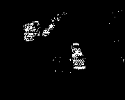
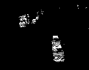
The frame rate for this traffic sequence is about 5 frames/second. The camera was mounted on a tripod on a bridge, so the background is static. If the purpose of the system is to monitor the traffic, the starting point is to separate the vehicles from the background. A good stab at this can be made using image differencing: we form pixel-by-pixel differences between each image and its predecessor, and identify regions where the grey-level changes most between frames.
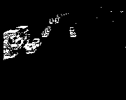
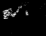
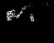
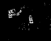
The following code demonstrates this idea. It forms each difference in turn, and then thresholds the differences so that we can see the places where the grey-level has changed by more than 20 units. In a real system, this threshold would be set dynamically, perhaps by reference to a histogram of the differences.
    vars read_to_float = sunrasterfile
        <> float_byte(% false, false, 0, 255 %);  ;;; see HELP *CLOSURES
    filesin(read_to_float, fname, 2, '.ras', 1, 1, 10) -> images;
    vars diffimage, lastimage;
    vars thresh = 20;            ;;; threshold for display
    images() -> lastimage;       ;;; get first image
    for image from_repeater images do
        float_arraydiff(image, lastimage, lastimage) -> diffimage;
        float_threshold2(1, -thresh, 0, thresh, 1, diffimage, diffimage)
            -> diffimage;   ;;; threshold the differences
        rci_show(diffimage) -> ;
        image -> lastimage;
    endfor;
(Final three images omitted here)
(If you want to clear some of these images from the screen later, you can click on each one as usual, or get rid of the last 9, say, with
rci_show_destroy(9); ;;; remove last 9 pictures
but do not do this till you have read the next paragraph.)
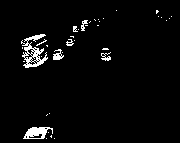
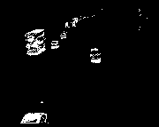
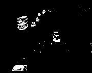
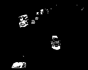
As you can see, one problem with this technique is that the grey level changes both where the vehicle was in the last image and where it is in the current image. Thus there is a kind of double view of each vehicle. One way to tackle this is to take differences from a reference image, which represents the background only of the scene. In general, producing a reference image is quite delicate, because it has to be continuously updated to allow for changes to the illumination as the sun moves and the weather changes, and to incorporate other slow changes, whilst not including any vehicles in the background even if they stop for a time.
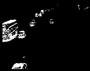
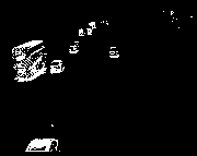
An approximate reference image for the scene, obtained simply by averaging a longer sequence of 700 frames, is available, and the following code demonstrates the result of taking differences with the reference image instead of the previous image.
    vars refimage;
    read_to_float(fname <> '_base.ras') -> refimage;
    filesin(read_to_float, fname, 2, '.ras', 1, 1, 10) -> images;
    for image from_repeater images do
        float_arraydiff(image, refimage, image) -> diffimage;
        float_threshold2(1, -thresh, 0, thresh, 1, diffimage, diffimage)
            -> diffimage;   ;;; threshold the differences
        rci_show(diffimage) -> ;
    endfor;
(Final four images omitted here)
The binary image sequence now looks considerably cleaner, though there is still some noise present. The static car at the bottom of the image, not shown by the successive differences, now appears, and segmentation of the moving vehicles from the background is reasonable. Various techniques could be applied to tidy the results further: isolated pixels could be removed, and morphological operations such as dilation and erosion used to consolidate the regions. Individual vehicles can be isolated to some extent using the kind of clustering approach provided in the *APPBLOBS library.
Further analysis of a traffic sequence such as this can take various directions. One way is to infer the 3-D structure of the road surface from the changes in size of the vehicle "blobs" in the binary images. This geometrical information than then be used to refine the processing of the images. Another important approach is to use knowledge about the way vehicles tend to move to carry out expectation based processing - computation can be focused on those parts of the image where we expect to find a vehicle, and the bottom-up data from the image can be combined with predictions from a 3-D model of the moving vehicles, preferably within some rigorous statistical framework.
There is not room to explore this kind of problem further at this point; instead, we will move on to some other kinds of motion information. You might want to clear the screen of images now with
rci_show_destroy("all");
You are used by now to the idea of images as 2-D structures, with x and y coordinates. It is sometimes helpful to think of an image sequence as a 3-D structure, with time, t, as the third dimension. Instead of thinking of an image sequence as a set of separate images, we can view it as occupying a block of space-time, something like this:
                             ------------------------------
                            /----------------------------/|
                           /----------------------------/||
                          /----------------------------/|||
        / t              /----------------------------/||||
       /                /----------------------------/|||||
      /                /----------------------------/||||||
     /                /----------------------------/|||||||
    ----------->     ------------------------------||||||||
    |         x      |                            ||||||||-
    |                |                            |||||||/
    |                |                            ||||||/
    |                |                            |||||/
    V y              |                            ||||/
                     |                            |||/
                     |                            ||/
                     |                            |/
                     ------------------------------
Here, the t axis is supposed to be at running away from you at right-angles to the x and y axes.
The division of time into frames is like the division of the spatial dimensions of the image into pixels.
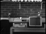
We will explore this idea by using it to look at an image sequence from a moving camera. First, the sequence displayed conventionally:
    0 ->> rci_show_x -> rci_show_y; ;;; start display at top left
    popvision_data dir_>< 'trolleyA' -> fname;
    filesin(sunrasterfile, fname, 3, '.ras', 1, 1, 20) -> images;
    for image from_repeater images do
        rci_show(image) ->
    endfor;
(Intervening 18 images omitted here)
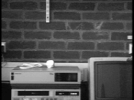
You can see that the camera is gradually approaching the objects on the bench. Each image is a slice through the x-y-t block at a particular value of t.
Now we will look at a slice at a constant value of x, displaying the intensity as a function of y and t. The dots in the figure below show two edges of the slice.
                             -------------------.----------
                            -------------------.----------|
                           -------------------.----------||
                          -------------------.----------|||
        / t              -------------------.----------||||
       /                -------------------.----------|||||
      /                -------------------.----------||||||
     /                -------------------.----------|||||||
    ----------->     -------------------.----------||||||||
    |         x      |                  .         ||||||||-
    |                |                            |||||||-
    |                |                  ^         ||||||-
    |                |                  |         |||||-
    V y              |                  -- x = 142||||-
                     |                  .         |||-
                     |                  .         ||-
                     |                  .         |-
                     ------------------------------
We arbitrarily choose an x value of 142, through the centre of the monitor screen to the right of the image. There are only 20 frames in the sequence, so to keep the slice a reasonable shape we will compress the y range down to 50 pixels. The code that follows sets up an array to receive the t-y slice, then copies the x = 142 column from each image into the appropriate t column of the slice array, using *arraysample.
    vars ty_slice = newsarray([1 20 1 50]);     ;;;
    filesin(sunrasterfile, fname, 3, '.ras', 1, 1, 20) -> images;
    vars t = 1, x = 142;
    for image from_repeater images do
        arraysample(image, [^x ^x 1 143], ty_slice, [^t ^t 1 50],
            "smooth") -> ;
        t + 1 -> t;
    endfor;
We can inspect the results with
    5 -> rci_show_scale;        ;;; show it larger, as only 20 x 50
    rci_show(ty_slice) -> rc_window;    ;;; we need the window later
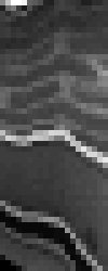
In the image now displayed, the axes are:
                                   t
                    ---------------->
                    |
                    |
                    |
                    |
                  y |
                    V
The clearest features are the bright traces produced by the top and bottom of the monitor, across the middle and bottom of the t-y plot. Notice how the traces diverge as time increases, corresponding to the growth in size of features in the original image sequence. In addition, there is a kink at the central frame, corresponding to slight change in the camera's motion at this point.
In practical computer vision, the use of explicit space-time representations like this is rare at present. However, as in many branches of physics and mathematics, space-time is a valuable conceptual tool, and can help in the development of algorithms.
One very important measurement can be made immediately from the space-time plot. The traces of the top and bottom of the monitor screen diverge at a definite rate. It is possible to calculate from this rate that the camera is likely to crash into the monitor after about another 40 frames of the sequence - and this calculation can be done without knowing anything about the size or distance of the monitor or the speed of the camera. (We do have to assume that the camera will continue its approach without changing speed.) We thus have an estimate of the likely time to collision on the basis of very simple measurements. This "time to contact under constant velocity" is a quantity likely to be highly relevant to controlling a mobile robot.
The calculation is as follows. Towards the end of the sequence, the size of the monitor screen increases by about 0.5 pixels per frame (using the large pixels in the t-y plot). Near the end of the sequence, the size of the monitor image, in the same units, is about 20 pixels. The size divided by the rate of expansion, 20 / 0.5, gives the number of frames left before collision is likely to occur.
(To verify these very approximate measurements, mark a few points on the t-y plot:
    rci_show_setcoords(ty_slice);
    'red' -> rc_window("foreground");   ;;; mark points in red
    rci_drawpoint(13, 26);      ;;; top at start
    rci_drawpoint(13, 43);      ;;; bottom at start
    rci_drawpoint(19, 30);      ;;; top at end
    rci_drawpoint(19, 50);      ;;; bottom at end
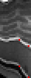
This shows that from frame 13 to frame 19, the image has grown from about 43-26 = 17 pixels to about 50-30 = 20 pixels. Three pixels growth in 6 frames is 0.5 pixels/frame. For real applications, the measurements would be made more carefully.)
The equation used above can be summarised as:
 time to contact under constant velocity
        (in frame intervals)

                        Size of image of object
                    =  --------------------------
                       Rate of expansion of image

                                 1
                    =  -------------------------
                       Relative rate of dilation
This relationship has been examined in some detail by psychologists, and it has been proposed as one of the mechanisms by which people and animals might time their actions. Observations, for instance of gannets diving into the sea and of people punching falling balls, have tended to confirm that this ratio (sometimes denoted by the Greek letter tau), might well be used for timing in some circumstances. For details of the experiments and derivations of the relationship, see Bruce & Green (1985), Lee (1980) and Lee & Young (1985). (Full references in TEACH * VISION.)
There is one caveat: the method is only accurate for objects close to the direction of travel, and that are not themselves rotating. These restrictions are true for many situations of interest, but the final section below will indicate how the idea can be generalised.
Estimates of the rate of expansion are not usually made directly from the space-time representation. One of the more successful recent methods has been to track closed contours in the image sequence using a snake or active contour mechanism. The area enclosed by the snake, rather than any single dimension, can be used to give a reliable measure of the expansion rate.
So far, we have looked at two special cases: the motion of individual objects in view of a fixed camera, and approach directly towards a surface. We need to go beyond these to have a general way to describe image change with time. For this, the central idea is that of the optic flow field.
Here, the term is used to mean the velocities of image features at a given point in time. (This is not strictly correct: the term ought to be used to describe the optic array rather than the image, and can also denote image changes over extended periods of time, but we will stick with the simpler usage.) Optic flow is to motion, roughly, what binocular disparities are to stereo vision - see TEACH VISION5.
Optic flow patterns are characteristic of different kinds of movement. For example, the optic flow field for the approach sequence in the previous section looks schematically like the display generated as follows:
    1 -> rci_show_scale;
    vars bounds = [1 192 1 142];        ;;; same size as previous array
    vars flowproc = first_order_flow(% 120, 50, 0.08, 0, 0, 0 %);
    display_flowproc(flowproc, bounds, 1, 10, false) -> rc_window;
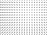
Each line represents an optic flow vector. The length and direction of the line indicate the speed and direction of motion of an image feature at the position of the dot. (For details of the procedures used here see HELP * FIRST_ORDER_FLOW and * DISPLAY_FLOW. These procedures are only being used as convenient ways of generating the diagrams, and understanding the code above is not important.)
The flow-field displayed is a dilating flow-field with a focus of expansion at the coordinates (120, 50). A focus of expansion is present in flow fields where the camera is moving through a static environment and is not rotating as it moves; it indicates the direction of heading of the camera, that is the point at which collision will occur if the camera keeps moving in a straight line. Note how the flow speed, indicated by the length of the vector lines, increases with distance in the image from the focus of expansion. In fact, the speed divided by this distance is a constant, and is just the (relative) rate of dilation of the image, used above to estimate time-to-collision.
Other situations produce different flow fields. For a camera moving sideways (regarding the direction of view as "straight ahead"), and viewing objects that are all about the same distance away (or a plane at right angles to the line of sight), the flow field is approximately uniform, roughly like that generated by:
    vars flowproc = first_order_flow(% 96, 10000, 0, 0.0005, 0, 0 %);
    display_flowproc(flowproc, bounds, 1, 10, rc_window) -> ;
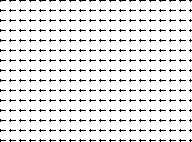
This is also close to the flow field generated by a rotation of the camera about the y-axis (a panning motion in cinematography), and in practice it can be difficult to separate out the two kinds of flow without additional information.
For a camera moving forwards over a planar ground surface, the flow field is roughly like this:
    false -> popradians;            ;;; Theta in degrees
    vars flowproc = first_order_flow(% 96, 0, 0.04, 0, 0.02, 90 %);
    display_flowproc(flowproc, bounds, 1, 10, rc_window) -> ;
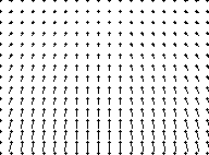
where the horizon is at the top of the window, whilst for a camera moving sideways over the ground, for instance a camera looking out of the side of a train, it is like:
    vars flowproc = first_order_flow(% 96, 0, 0, 0.02, 0.02, -45 %);
    display_flowproc(flowproc, bounds, 1, 10, rc_window) -> ;
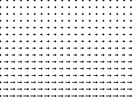
If there are independently moving objects present (as with the traffic example), or surfaces at differing distances or different orientations, then the flow field will be more complex, with different regions showing different patterns.
It is surprisingly difficult to measure optic flow accurately. One approach is to identify individual image features, such as grey-level corners, and track them from frame to frame. It is then necessary to solve something like the stereo correspondence problem; how difficult this is depends on the frame interval. This kind of approach produces a sparse set of flow vectors, as vectors are only defined for definite features. The snake-based method mentioned above is proving a powerful technique for tracking large-scale features, which may also be distorting in particular ways as the movement progresses, and the information implicit in the snake's shape can avoid the need to calculate explicit flow vectors.
There is a different class of methods based on the use of local measurements of the spatial and temporal structure of the image sequence. These attempt to produce a dense set of flow vectors, with a vector defined for every pixel. We will discuss one of the simplest of these approaches, due to Horn & Schunck (1981; see TEACH * VISION).
The Horn-Schunck method makes use of the simplest local structure that can give information about motion: the grey-level gradient. This allows extremely simple low-level processing to be used, at the expense, as we shall see, of some extra processing to resolve ambiguities. (TEACH VISION3 describes the spatial grey-level gradient.)
The basic idea is as follows. Suppose that there is a grey-level gradient of 2 units per pixel in some small region of the image. If the gradient direction is along the x-axis, the grey-levels in the region might be:
   --------------------------
   | 23 | 25 | 27 | 29 | 31 |
   |----+----+----+----+----|      ----------------->
   | 23 | 25 | 27 | 29 | 31 |      g.l. gradient is
   |----+----+----+----+----|      2 units/pixel in
   | 23 | 25 | 27 | 29 | 31 |      this direction
   --------------------------
Now suppose that in the same rows and columns of the image, but in the next frame in sequence, the values are
   --------------------------
   | 17 | 19 | 21 | 23 | 25 |      ------------------>
   |----+----+----+----+----|      Image has moved 3
   | 17 | 19 | 21 | 23 | 25 |      pixels this way.
   |----+----+----+----+----|      g.l's at corresponding
   | 17 | 19 | 21 | 23 | 25 |      pixels have decreased by 6
   --------------------------
You can see that a motion of 3 pixels to the right accounts for the new values. The change in grey-level at corresponding pixels is 6 units (e.g 27 to 21 in the central pixel). If the spatial grey-level gradient is 2 units per pixel, and we shift the values by 3 pixels, then the total change is 2 x 3 = 6. We can manipulate this to say that
 distance moved per frame

            Change in grey-level at corresponding pixels
         =  --------------------------------------------
                   Spatial grey-level gradient
or in this case 6 (the temporal gradient) divided by 2 (the spatial gradient) gives 3 (the amount of motion). A great advantage of the approach is that it is easy to measure these spatial and temporal gradients, by combining smoothing and differencing operations.
This argument makes a big assumption - the constant intensity assumption - that the change in grey-level is entirely due to motion. In other words, the grey-levels "move along with" the motions of the images of physical features. This is often not true - for instance specular reflections and highlights do not behave in this way, and the illumination can change - but it is a good enough assumption to make a reasonable starting point for estimating the flow.
There is a further problem. In the example above, a motion along the y-axis will not have any effect on the grey levels, because it maps like values onto one another. Thus we only have information about motion along the x-axis in this case, or in general along the grey-level gradient. This component of motion is sometimes called the edge motion; it is at right-angles to the local edge direction.
This effect is a manifestation of what is known as the aperture problem, because it is a result of considering a local region of the image only. If we used information from a larger region, rather than looking through a small window at the image, the extra structure would allow to infer the other component of motion. Horn & Schunck tackled the aperture problem by arguing that adjacent regions of the image should usually have similar motions, because the regions are usually images of adjacent parts of the same physical surface. If a nearby part of the image had a grey-level gradient along the y-axis, then this would constraint the other component of the local flow vector.
This boils down to two requirements:
Horn & Schunck proposed an iterative algorithm which yields flow fields that satisfy these conditions. Although the algorithm was derived using a fairly sophisticated analysis, it amounts in effect to adjusting an estimated flow field to satisfy each of the conditions in turn more closely. On each iteration, the algorithm:
This iterative approach to satisfying constraints belongs to the class of algorithms known as relaxation algorithms.
Does this work? We can try it on the last two images from the approach sequence:
    vars image1 = read_to_float(fname <> '019.ras');
    vars image2 = read_to_float(fname <> '020.ras');
    rci_show(image1) -> ;
    rci_show(image2) -> ;
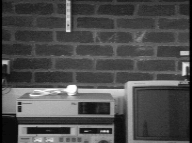

which can be processed and the flow field on each iteration displayed with
    max(popmemlim, 1e6) -> popmemlim;       ;;; may need more memory
    false -> rc_window;
    vars hs = horn_schunck(image1, image2, 2, 2, 0.005);
    vars u, v;          ;;; will be arrays holding flow vec comps
    repeat 10 times
        hs() -> (u, v);
        display_flow(u, v, 3, 11, rc_window) -> rc_window
    endrepeat;
 (After 1 iteration)
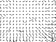 (After 10 iterations)
After the first iteration, the flow vectors show pure edge motion, so tend to lie along the x- and y-axes, because the edges in the image tend to be aligned this way. As the iteration proceeds, smoothing moves the vectors round, and we end up with something that resembles, at least a little, the "ideal" dilation flow field demonstrated earlier. Of course, it is much more noisy, and a few of the vectors are entirely incorrect, but the idea is clearly working to some extent.
For more details of the program used here, and another example of it in use, see HELP * HORN_SCHUNCK. You could also try applying it to some frames of the traffic sequence. Note that the program is faster than it seems, as most of the time spent running the example above goes in producing the display.
Many variations on the method of Horn & Schunck have been proposed. One of its chief problems, apart from sensitivity to noise, is that the smoothing step blurs what ought to be sharp jumps in the flow field, at the edges of objects at different depths for instance. This can be addressed by allowing explicit discontinuities in the vector field, and also by using more careful forms of smoothing that take account of the amount of information available to constrain the different components of the vectors. Some related approaches combine vectors round closed contours (e.g. Hildreth, 1984; full reference in TEACH * VISION), so that the problem of propagating the flow into large uniform regions is avoided.
Relatively recently, the gradient-based method has been generalised to filter-based methods. These use local operators with a more complex structure than the simple differencing operators needed to estimate gradients. Such operators yield a richer description of the local grey-level structure in space-time, and the methods are producing promising results.
We have already mentioned that approach to a surface leads to a flow-field with a simple dilational pattern. If we are willing to assume that the flow-field we have measured has this form, then it is straightforward to estimate the position of the focus of expansion and the rate of dilation. This can be done on our existing flow estimates from the end of the approach sequence with
    vars D, x0, y0;
    solve_dilation(u, v) -> (D, x0, y0); ;;; see HELP * SOLVE_DILATION
and the position of the focus of expansion shown with
    'red' -> rc_window("foreground");
    rci_show_setcoords(u);
    rc_filledcircle(x0, y0, 3);
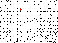
or on the original image
    rci_show(image1) -> rc_window;
    'red' -> rc_window("foreground");
    rci_show_setcoords(image1);
    rc_filledcircle(x0, y0, 3);
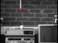
This indicates where collision will occur if the camera keeps moving with constant velocity, and assuming it is not rotating. In addition, the quantity D is the (relative) rate of dilation, the flow speed at each pixel divided by the distance from the focus of expansion. The inverse of this, as explained above, gives an estimate of the time to collision (measured in frame intervals). Printing this quantity:
    1/D =>
prints:
    ** 45.4131
shows a value of about 45 frame intervals to collision - in good agreement with the earlier estimate of 40 frame intervals made from the space-time plot.
In all this, we have treated the objects in view as if they all lie in the same vertical plane in front of the camera. Clearly we need a more general approach. There is a very large literature on this topic, and a wide variety of ways to proceed. Two of the main ones are now outlined, but a detailed analysis or demonstration is beyond the scope of this file.
If we assume that the world is rigid and the camera moves through it, and we obtain flow vectors for some features in the image, then it is possible, in principle, to work out how the camera is moving and also the relative depth of the scene features (i.e. points on surfaces in the world) associated with the flow vectors. This is known as solving the structure-from-motion problem, since the depths of objects, together with their image positions, give their full 3-D positions.
The motion of the camera at any instant can be described by a translation velocity and a rotation angular velocity. Each of these requires three numerical variables to describe it. For instance, the components of the motion along the three camera coordinates (see TEACH VISION5) describe the translation, and the rates of rotation about the three axes describe the overall rotation. There are thus 6 motion parameters that need to be found.
In addition, the depth (or distance from the camera) of each scene feature is unknown. Thus if we observe N flow vectors, there are N unknown depths. The total number of unknowns is therefore N + 6.
In fact, optic flow alone can never determine all of the translation parameters. Exactly the same optic flow can be produced by a small, close object moving slowly as by a large, distant object moving fast. There is a speed-scale ambiguity, which means that we can only determine the distances of the scene features relative to the translation speed, and vice versa. That is, we might as well assume the camera speed to be 1 unit per frame, and measure distances in these "units", whose actual size in inches or metres, remains unknown for now. This reduces the number of unknowns to N + 5, since there are only two independent translation parameters now.
Now, for each flow vector, we have two measurements: the x and y components of the vector, each of which depends on the N + 5 unknown parameters as well as position in the image. We therefore have 2N equations, and N + 5 unknowns. This suggests that for 5 or more flow vectors we ought to be able to solve the equations and find the structure and motion.
This turns out to be true in general, though the mathematics of the solution is not trivial. Certain configurations of points in space make the solution impossible, and it turns out that in general the solution is very sensitive to noise. In particular, rotation and sideways translation of the camera get confused in the presence of only very modest amounts of noise.
One way to tackle this sensitivity is to integrate the results of analyses extended over time. We may, for instance, assume that the camera motion is reasonably smooth, and use many frames to build up an accurate estimate of the structure and motion. Alternatively, we may use non-visual information, such as may be available from the drive system of a robot, to provide additional knowledge of camera translation or rotation, simplifying the problem enormously.
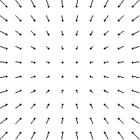
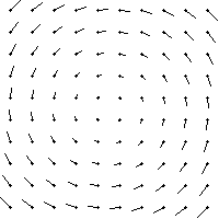
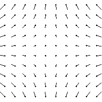
An alternative way to get information from motion is to assume that the flow in some small region of the image is the result of motion relative to a smooth patch of surface. In this region, we ignore the average flow, but look at the local relative pattern of the flow - the differential flow. This will be a combination of
dilation:
    vars flowproc = first_order_flow(% 100, 100, 0.1, 0, 0, 0 %);
    display_flowproc(flowproc, [1 200 1 200], 1,20,false) -> rc_window;
rotation:
    vars flowproc = first_order_flow(% 100, 100, 0, 0.1, 0, 0 %);
    display_flowproc(flowproc, [1 200 1 200], 1, 20, rc_window)
        -> rc_window;
the first component of shear:
    vars flowproc = first_order_flow(% 100, 100, 0, 0, 0.1, 0 %);
    display_flowproc(flowproc, [1 200 1 200], 1, 20, rc_window)
        -> rc_window;
and the second component of shear:
    vars flowproc = first_order_flow(% 100, 100, 0, 0, 0.1, 45 %);
    display_flowproc(flowproc, [1 200 1 200], 1, 20, rc_window)
        -> rc_window;
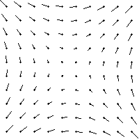
It is possible to analyse the local differential flow into these components, and hence to make inferences not only about time-to-collision, but also about the tilt and slant of the surface relative to the camera. Such information may well be as valuable for control of robot motion as a full solution of the structure-from-motion problem.
You should now:
Here are links to:
Copyright University of Sussex 1994. All rights reserved.