Discrete Dynamics Lab
return to: DDLab home - update summary - multi-Value - dd-life - 3d glider-guns

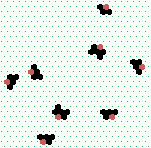
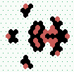
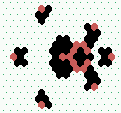
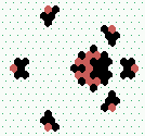
The spiral glider-gun rule, v=3 k=7
Further details and results relating to the paper:
Wuensche,A., A.Adamatzky, (2006),
"On spiral glider-guns in hexagonal cellular automata: activator-inhibitor paradigm"
to appear in International Journal of Modern Physics C (preprint online here)

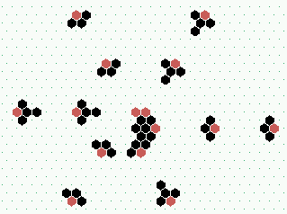
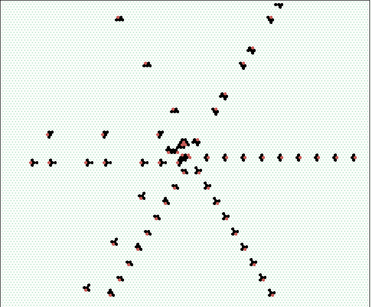
Fundamental structures in the spiral rule, which can be interpreted as a reaction-diffusion system (activator, inhibitor and substrate). Note also that the dynamics are symmetric — all phenomena can occur equally in any direction, or clockwise and anti-clockwise.

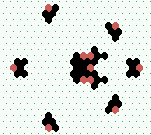
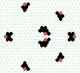
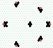
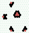
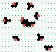
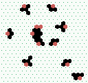
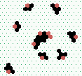
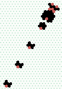
5 basic types of mobile gliders (G1-G5), all travelling NorthEast, in the direction of their "active" red heads.

2 types of static "eaters" (E1, E2),
E2 has "memory" on its outer shell

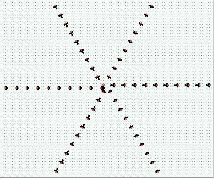
S1: high-frequency spiral glider-gun shooting G1 gliders, frequency=6

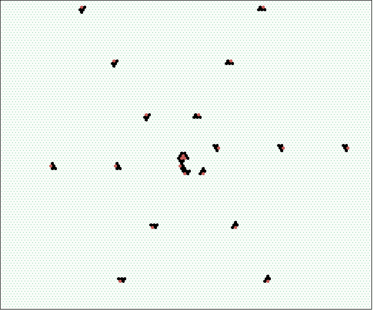
S2: low-frequency spiral glider-gun shooting G2 gliders, frequency=21


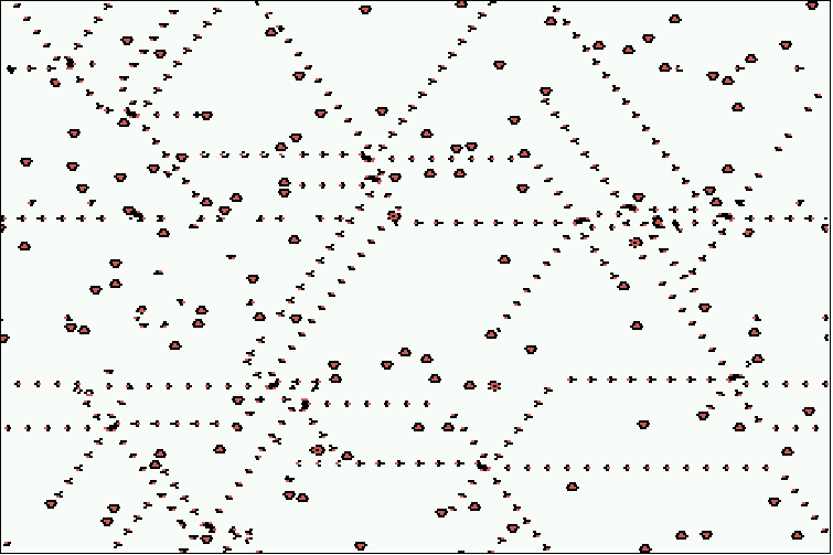
S1 and S2 spiral glider-guns, 120x120, click to enlarge

S1: high-frequency spiral glider-gun

S2 low-frequency spiral glider-gun

high and low-frequency spiral glider-guns interacting

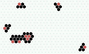
Polymer gliders and eaters
forming chains, aggregations and oscillators of arbitrary length, can exist in many combinations.

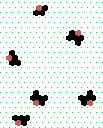
Various types of small 2-headed gliders heading NE.

Examples of linked eaters.

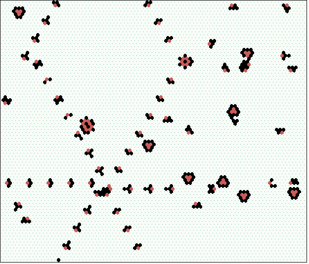
Snapshots of evolved systems, with gliders, glider-guns and eaters, forming quasi-stable circuits, click to enlarge.

snapshot 88x88

snapshot 250x250

72 single mutations to the spiral rule
36 are quasi-neutral. Click to enlarge. The initial state is the 88x88 snapshot above.
index
0-5
0

1

2

3

4

5

index
6-11
6

7

8

9

10

11

index
12-17
12

13

14

15

16

17

index
18-23
18

19

20

21

22

23

index
24-29
24

25

16

27

28

29

index
30-35
30

31

32

33

34

35


Pairwise collisions between basic gliders - some examples
Mutual annihilation 2→0
3
steps
3
steps
Conservation + Destruction 2→1
2
steps
2
steps
One glider bouncing off another 2→2
180° bounce
6 steps
120° bounce
7 steps
Reproduction
2→4
6
steps
2→6
10
steps
2→8
13
steps
2→6
15
steps
Creating eater E1
eater
E1
+ 4
gliders
10
steps

Memory - Glider interacting with eater E2
Write
Read

Creating spiral-glider guns S1 and S2 S1 spiral
glider-gun
S1 spiral
glider-gun
S2 spiral
glider-gun

mobile gliders-guns, some examples, with heading (moving head direction) indicated
heading NE
heading NE
heading NE
heading NE
heading NE
heading East

Building the spiral rule
The lookup table
v=3 cell-states (cell-values) [2, 1, 0] are represented by cell-colors: black, red, white in the examples above. A cell updates its state depending on the totals of [2s, 1s, 0s] in its neighborhood, size k=7 — the cell and its nearest neighbors on a lattice with hexagonal tiling. There are S = (vk - 1)! / (k!(v -1)!) possibilities, so 36 [2, 1, 0] sub-rules (and their outputs) set out in DDLab's format below. The output string defines the rule (also represented in hexadecimal).
 35                                  0 - rule-table index
  |                                  |
2:766555444433333222222111111100000000
1:010210321043210543210654321076543210
0:001012012301234012345012345601234567
  ||||||||||||||||||||||||||||||||||||
  000200120021220221200222122022221210 = 020609a2982a68aa64 in hexadecimal
The filename of the spiral rule in DDLab is v3k7w1.vco

k7 hex neighbourhood
The consequences of mutating the spiral glider-gun rule's lookup table
Each lookup table output (subrule) has two possible mutations, 72 in all, This table indicates the consequences of each mutation, and which subrules are quasi-neutral (+,-), and which are responsible for gliders (>). This relates to the neighborhood frequency histogram, the frequency of sub-rules in the evolving CA. A snapshot of each mutation is shown below.
              rule-table index
             /  totals: 2s+1s+0s=k=7
            /  /       rule-table
           /  /       / mutations  neighborhood frequency histogram
          / 2_1_0    /  2___1___0
         0: 0 0 7 : 0 > o   c   .  |||||||||||||||||||||||||||||| 85.7% =>
         1: 0 1 6 : 1 > o   .   o  |||||||||||| 0.7%
         2: 0 2 5 : 2   .   g   g  ||
         3: 0 3 4 : 1 + G   .   G  |
         4: 0 4 3 : 2 - .   G   G  :
         5: 0 5 2 : 2 - .   G   G  :
         6: 0 6 1 : 2 + .   G   G  :
         7: 0 7 0 : 2 + .   G   G  :
         8: 1 0 6 : 0 > c   c   .  |||||||||||||||||||||||||||||| 4.5% =>
         9: 1 1 5 : 2 > .   c   c  |||||||||||||||||||||||| 1.4%
        10: 1 2 4 : 2   .   g   g  ||||
        11: 1 3 3 : 1 + G   .   G  |
        12: 1 4 2 : 2 + .   G   G  :
        13: 1 5 1 : 2 + .   G   G  : 
        14: 1 6 0 : 2 + .   G   G  ||
        15: 2 0 5 : 0 > c   c   .  |||||||||||||||||||||||||||||| 2.3% => 
        16: 2 1 4 : 0 > o   c   .  ||||||||||||||||||||||| 1.3%
        17: 2 2 3 : 2   .   c   g  ||||
        18: 2 3 2 : 1 - G   .   G  || 
        19: 2 4 1 : 2 + .   G   G  |
        20: 2 5 0 : 2 + .   G   G  ||
        21: 3 0 4 : 0 > g   c   .  ||||||||||||| 0.8%
        22: 3 1 3 : 2 > .   c   g  |||||||||||||||||||||||||| 1.6% 
        23: 3 2 2 : 2   .   g   g  |||||| 
        24: 3 3 1 : 1   g   .   g  |||| 
        25: 3 4 0 : 2 - .   G   G  |
        26: 4 0 3 : 0   g   G   .  ||| 
        27: 4 1 2 : 0 > G   c   .  |||||||||| 
        28: 4 2 1 : 2   .   cg  g  ||
        29: 4 3 0 : 1   g   .   g  |||||||| 
        30: 5 0 2 : 0   G   c   .  ||  
        31: 5 1 1 : 0 > G   c   .  ||| 
        32: 5 2 0 : 2 - .   G   G  ||  
        33: 6 0 1 : 0   G   c   .  ||
        34: 6 1 0 : 0   G   cg  .  ||
        35: 7 0 0 : 0 - G   G   .  |
Key to mutations
G:quasi-neutral, g:related but different glider dynamics emerge c:chaotic, cg:tends to chaos but with gliders present o:order. 36 mutations and 15 sub-rules are wildcards, making no impact, or minimal impact on the dynamics. Sub-rules are marked as: +strong wildcards (9), weak wildcards (6), and >glider-critical (10)

The rule as a matrix
The rule can be represented more simply as an ij matrix as shown below, were i represents the number of 2s, and j the number of 1s. The number of 0s follows: 7-(i+j). The output of each sub-rule can be read off each ij. The matrix on the right shows: +:strong wildcards, and –:weak wildcards.
 
       the spiral glider-gun rule as a k=7 matrix

                j=1s              wildcards       
          0 1 2 3 4 5 6 7         -weak  +strong    
          ...............         
       0: 0 1 2 1 2 2 2 2         0 1 2 + - - + +  
       1: 0 2 2 1 2 2 2           0 2 2 + + + +   
       2: 0 0 2 1 2 2             0 0 2 - + +     
  i=2s 3: 0 2 2 1 2               0 2 2 1 -       
       4: 0 0 2 1                 0 0 2 1
       5: 0 0 2                   0 0 -
       6: 0 0                     0 0 
       7: 0                       -


neighbourhoods frequency histogram:
snaphot from DDLab
The rule as a k=6 outer-totalistic rule
The same rule can be expressed as a k=6 outer-totalistic rule, which consists of three centre-rules, one for each state (or value [2, 1, 0]) of the central cell, c. Each centre-rule has 28 sub-rules, which are shown in the DDLab format, and tabular and matrix form below, indicating strong (+), and weak (-) wildcards.
       28                          0 - rule-table index
        |                          |
    | 2:6554443333222221111110000000
   v| 1:0102103210432105432106543210
    | 0:0010120123012340123450123456   hexadecimal     filename in DDLab
        ||||||||||||||||||||||||||||   --------------  ----------
    | 0:0002001220212002212202221210 - 020689829a2a64  w1otc0.vco
   c| 1:0201202122221202221222222121 - 2189aa62a6aa99  w1otc1.vco
    | 2:0002001200212202212002221220 - 020609a2982a68  w1otc2.vco

      3 k=6 outer-totalistic rules
      rule table index 
     /  totals: 2s+1s+0s=k=6         3 k=6 outer-totalistic matrices
    /  /      rule tables  
   /  /     ----------------                j=1s         wildcards 
  / 2_1_0   C=2   C=1    C=0            0 1 2 3 4 5 6    -weak  +strong 
 0: 0 0 6 : 0     1      0              .............
 1: 0 1 5 : 2     2      1      c=2  0: 0 2 2 1 2 2 2    0 2 2 + - - +   
 2: 0 2 4 : 2     1+     2           1: 0 0 2 1 2 2      0 0 2 - + +
 3: 0 3 3 : 1+    2-     1+          2: 0 2 2 1 2        0 2 2 1 -
 4: 0 4 2 : 2-    2-     2-     i=2s 3: 0 0 2 1          0 0 2 1
 5: 0 5 1 : 2-    2+     2-          4: 0 0 2            0 0 -
 6: 0 6 0 : 2+    2+     2+          5: 0 0              0 0
 7: 1 0 5 : 0     2      0           6: 0                0
 8: 1 1 4 : 0     2      2           
 9: 1 2 3 : 2     1+     2           
10: 1 3 2 : 1-    2+     1+         
11: 1 4 1 : 2+    2+     2+     c=1  0: 1 2 1 2 2 2 2    1 2 + - - + +
12: 1 5 0 : 2+    2+     2+          1: 2 2 1 2 2 2      2 2 + + + +
13: 2 0 4 : 0     0      0           2: 0 2 1 2 2        0 2 - + +
14: 2 1 3 : 2     2      0      i=2s 3: 2 2 1 2          2 2 1 -
15: 2 2 2 : 2     1-     2           4: 0 2 1            0 2 1
16: 2 3 1 : 1     2+     1-          5: 0 2              0 -
17: 2 4 0 : 2-    2+     2+          6: 0                0
18: 3 0 3 : 0     2      0           
19: 3 1 2 : 0     2      2          
20: 3 2 1 : 2     1      2            
21: 3 3 0 : 1     2-     1      c=0  0: 0 1 2 1 2 2 2    0 1 2 + - - +
22: 4 0 2 : 0     0      0           1: 0 2 2 1 2 2      0 2 2 + + +
23: 4 1 1 : 0     2      0           2: 0 0 2 1 2        0 0 2 - +
24: 4 2 0 : 2-    1      2      i=2s 3: 0 2 2 1          0 2 2 1
25: 5 0 1 : 0     0      0           4: 0 0 2            0 0 2 
26: 5 1 0 : 0     2-     0           5: 0 0              0 0
27: 6 0 0 : 0-    0      0           6: 0                0


k6 outer-totalistic
hex neighbourhood


back to the DDLab home page
April 2006 -- Last modified: June 2009