

| Discrete Dynamics Lab |
|
The multi-value version of DDLab
allows network elements to have a value range v anywhere from 2 to
8. All DDLab functions (as described in the manual)
have been generalised for multi-value,
including setting rules and initial states, attractor basins including
compression, space-time patterns,
filtering, frozen cells, graph layout,
density plots (each density is shown),
look_up histogram, input-entropy, entropy-density plots,
automatic classification and samples of
glider rules (include in dd_extra.zip), the reverse algorithms for
CA, RBN and random maps, the Z and lambda
parameters, learning algorithms, the meta-graph, canalising,
the Derrida plot, and damage spread.
Some new functions include: Post functions, symmetric and
k-totalistic rules for 1d, 2d and 3d, "un-slanting" 1d space-time patterns,
and hexagonal neighborhoods/lattice. Click here for a summary of changes. Click here for examples and details of DD-Life, families of "Life"-like and other complex 2d and 3d CA rules Click on the images below to see them full size. |

|
| The basin of attraction field of a n=6, k=3 CA with a value range v=3 (i.e. values 0,1,2 colored white, red and black). The look-up table is 222211010010021221122111221 with a Z-parameter=0.37037. Just the 5 non-equivalent basins are shown from a total of 8, and non-equivalent attractor states are shown as 2d 3x2 patterns. State-space = 3^6 = 729. |

|
| The basin of attraction field of a n=8, k=3 CA with a value range v=3 (i.e. values 0,1,2 colored white, red and black). The look-up table is 020120102021201201011011022 with a Z-parameter=0.7037. Just the 7 non-equivalent basins are shown from a total of 17, and one attractor state in each basin is shown as 2d 4x2 pattern. State-space = 3^8 = 6561. |

|
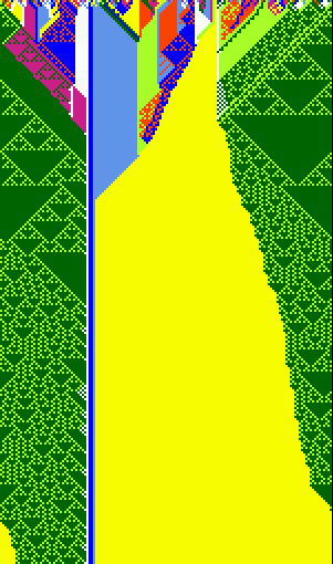
| 1d space-time patterns from random initial states. n=150, v=8, k=4, 1d CA, showing the evolution of a generalised Altenberg rule, where the probability of a look-up table output is equal to the frequency of values in its neighborhood. |
|

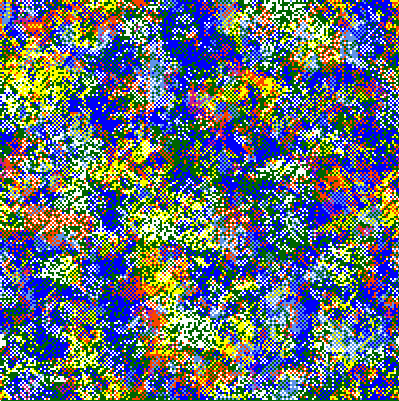
| Evolved 2d patterns from random initial states. n=200x200, v=8, k=4, 2d CA, for two generalised Altenberg rules, where the probability of a look-up table output is equal to the frequency of values in its neighborhood. |
|
|
|
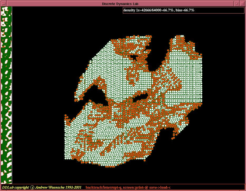
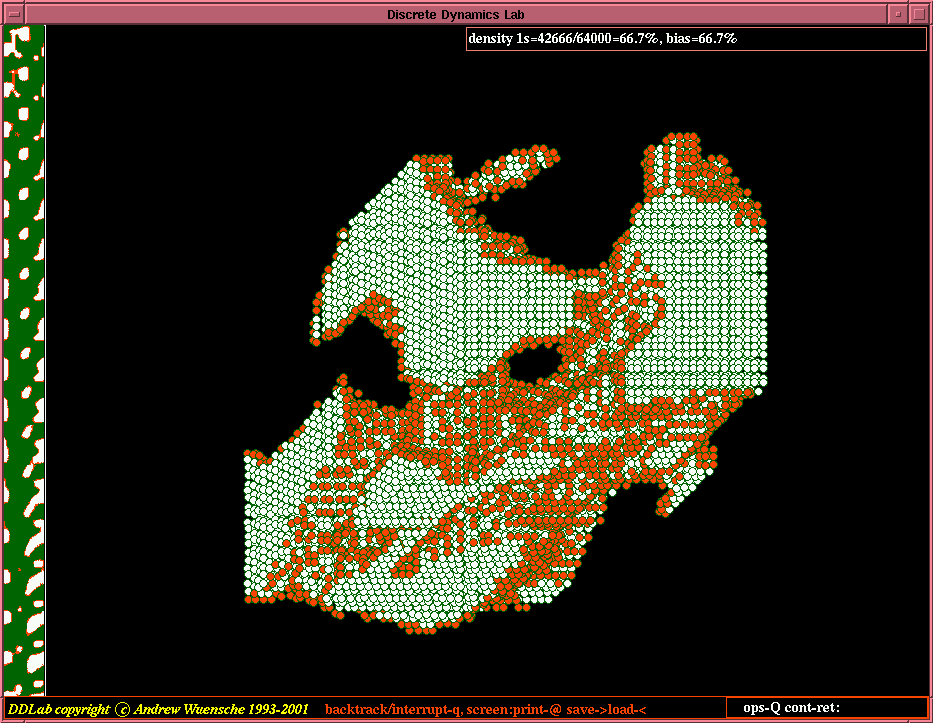
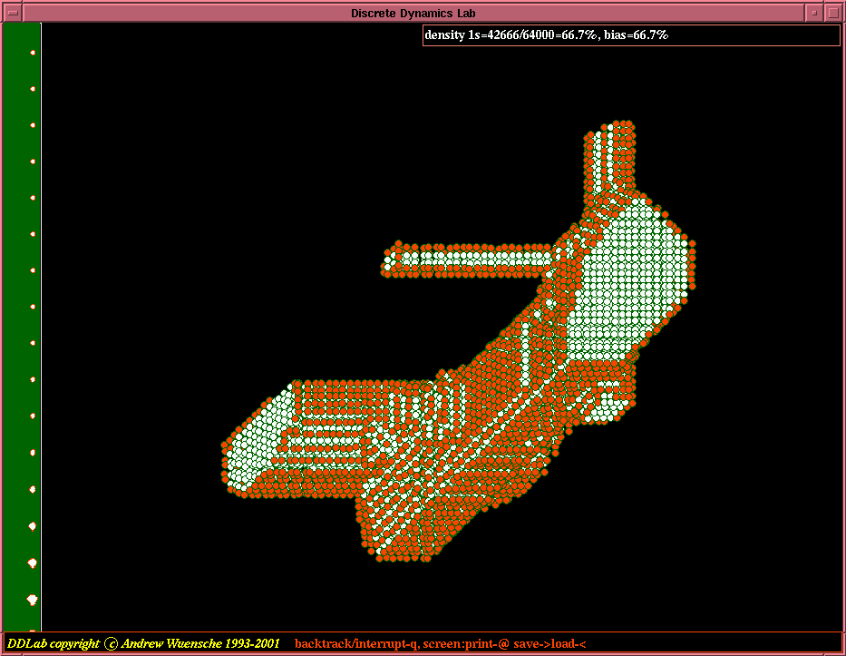
| A 3d, 40x40x40, v=3, k=7, CA, values 0,1,2 colored white, red and black, showing the evolution according to the totalistic rule, code 2222122111101100000. Horizontal x-sections of the 3d network are shown on the left. | ||

| 
| 
| 
| 
|
| An example of the space-time patterns of a 1d symmetric rule, v=8, k=2, n=150. The seed is a single 6 (yellow) in a uniform background of 7s (white). There are 670 time-steps in each panel, which follow on from each other. In the 5th panel the dynamics reaches the all 4s (light blue) point attractor. This is a "symmetric/legal" rule, where "symmetric" means that reflected neighborhoods have the same output in the lookup table, and "legal" (after Wolfram) means a symmetric rule where the uniform neighborhoods output their corresponding color (i.e. 000->0, 111->1, 222-2 etc). Setting such rules at random is a new feature in multi-value DDLab. The example also illustrate another new feature, the ability to "un-slant" k=2 (or any even k) space-time patterns by rotating successive rows by 1/2 cell width. This maintains the appearance of symmetry for even k and makes a k2 system equivalent to a triangular lattice. | ||||
| 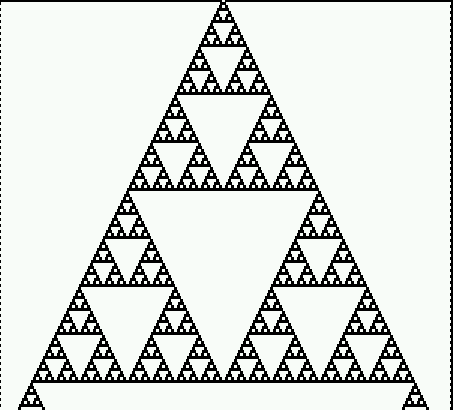
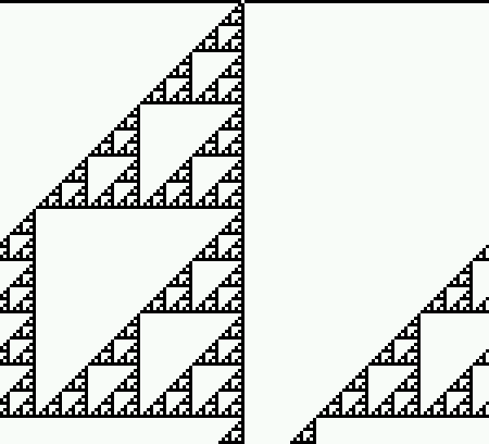
| The "un-slant" option can be applied irrespective of k. Odd k rules are sometime effectively even k rules, such as the v2k3 cluster of equivalent rules 60,195,102,153 (the equivalent v2k2 cluster is 6,9). On the left is rule 153 as normally seen, on the right "un-slanted". n=150, 197 time-steps from seed of a single 1 (white) in a background of 0s (black). |
| 
| 
| 
| 
|
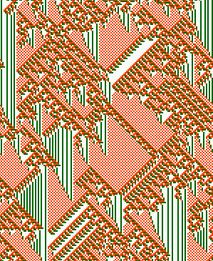
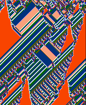
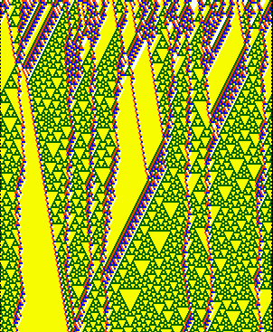
| v3k3 | v4k2 | v4k3 | v4k3 | v5k2 |
| Examples of multi-value complex rules found by the automatic classification method, and included in multi-value DDLab. Note that the k2 examplea have been "un-slanted" (see above). n=150, 183 timesteps from random seeds. | ||||
| 
| 
|
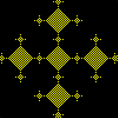
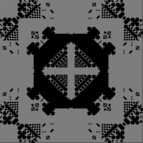
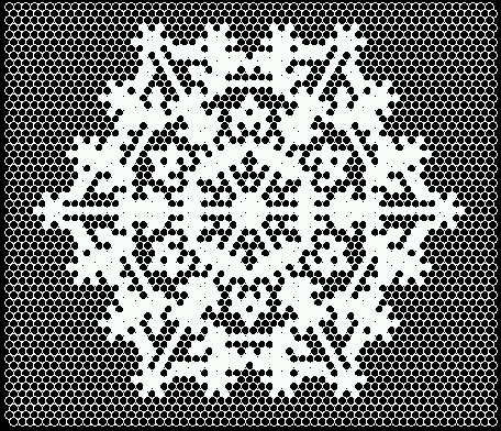
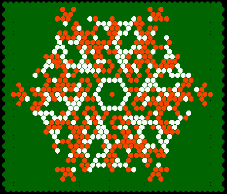
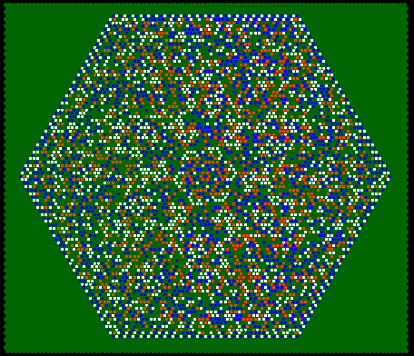
| v2, k4, 40x40 | v2, k4, 250x250, changing the symmetric rule on-the-fly | v2, k6, 60x60 shown in hexagonal graph layout |
| 
| 
|
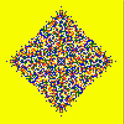
| v3, k6, 40x40 shown in hexagonal graph layout | v4, k7, 100x100 shown in hexagonal graph layout | v5, k5, 100x100 |
| Examples of the evolved space patterns of 2d symmetric rules. Starting from a symmetric pattern the symmetry must be conserved. | ||
| 
| 
| 
|
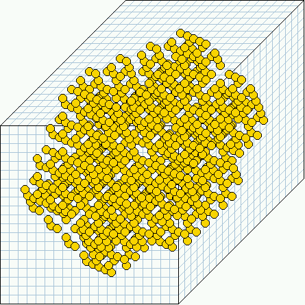
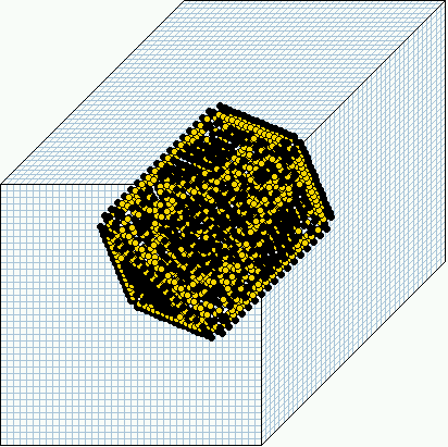
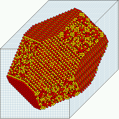
| v2, k6, 20x20x20 | v4, k6, 40x40x40 | v5, k6, 30x30x30 | v4, k7, 40x40x40 |

| |||
| v5, k6, 18x18x18, showing successive horizontal slices from left to right. | |||
| Examples of the evolved space patterns of 3d symmetric rules. Starting from a symmetric pattern the symmetry must be conserved. | |||