Introduction
Welcome to the information page. To view a specific section, please click on any of the links on the sidebar.
The sections on neurons and the neuron models below are designed to be accessible to beginners, and therefore are not comprehensive. For greater detail or more information, follow any of the links below
Using The Simulations
The simulations are generally self explanatory, and it is encouraged to play around with the features to understand them. All of the input parameters have a descriptive popover box when hovering, to explain more about them. To get started, simply change any of the input parameters and press the 'Submit' button. For further information on how to do anything, read the relevant section below.
Changing the Parameters
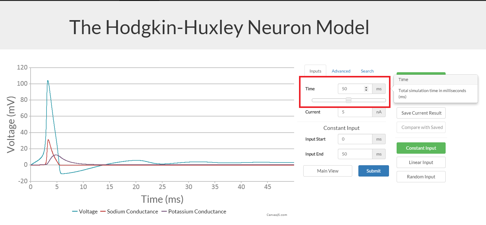
To change any of the input parameters, click on the desired input box, and simply input a number using your keyboard. Alternatively, you can increase or decrease the current input using the arrows in the box, mouse wheel, or by using the slider bar which appears below the input box when clicked. When hovering over the input box, more information about the parameter will appear in a popup box
Input Current Types
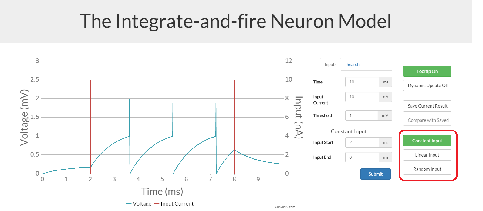
The three types of input current are constant, linear, and random. In all three types the start and end of input can be set, as well as the maximum input. To select input type click on the relevant button in the 'options' sidebar.
In constant input, the current will be set at the maximum input current for the whole duration from input start to end. Outside of this the current will be 0 nA.
In linear input, the current starts at 0 nA, and increases linearly to the maximum input current over the course of the input duration. After the end of input, the current remains at the maximum value until the end of the simulation.
In random input, between input start and end, the current is randomised. The minimum input can also be set here, with a default of 0 nA. The range of random values is always between the minimum and maximum. The other thing that can be set here is the change rate, which has a default of 1 ms. This means the random value changes every 1 milliseond unless changed.
Dynamic Update
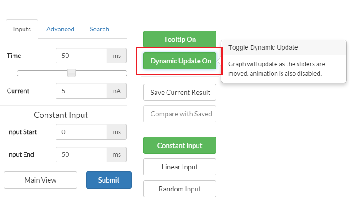
To change the graph to update dynamically, click the ' dynamic slider on/off' button. This now means that when using the sliders under the input boxes, the graph will update as the slider does. This is very useful for seeing the effect of one of the inputs, or for finding the desired amount quickly. This option also disables animation.
Choosing the desired output
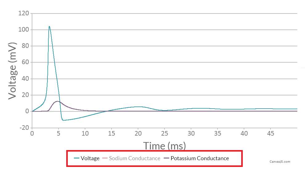
The main output type is Voltage. Depending on the simulation, you can also view input current, sodium conductance, and potassium conductance. These can be viewed in any combination. To change desired output, click on the legend to toggle the chosen value. This is particularly useful when comparing two seperate inputs (see comparing inputs section.)
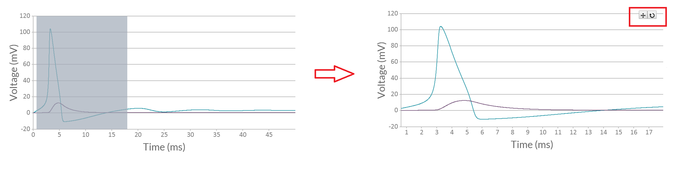
Zooming and panning
To zoom in on the graph, click and drag across the desired section. The graph will automatically adjust to the scale of the new section. To move along the graph, click on the arrowed icon at the top right corner, and then drag your cursor to either the left or right as desired. You can switch back to zooming by clicking on the magnifying glass icon. To reset the graph to the original view, click the refresh icon.
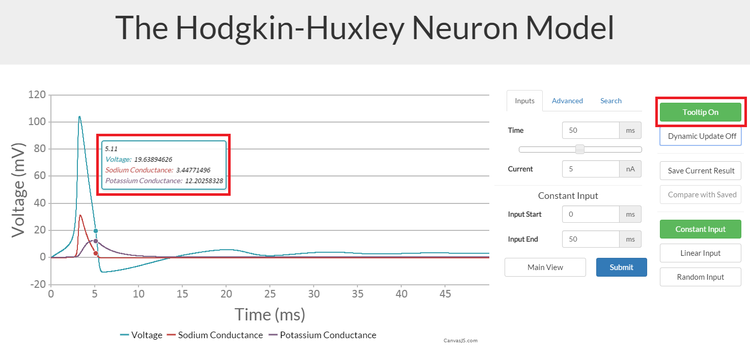
Viewing the tooltip and exact output values
To see the exact value of any part of the output, simply hover over the desired part of the graph with your cursor and a tooltip will appear. The tooltip will show the timestep, and exact values for all the outputs. This is especially helpful when comparing multiple inputs.
To disable this feature, uncheck the box in the options menu.
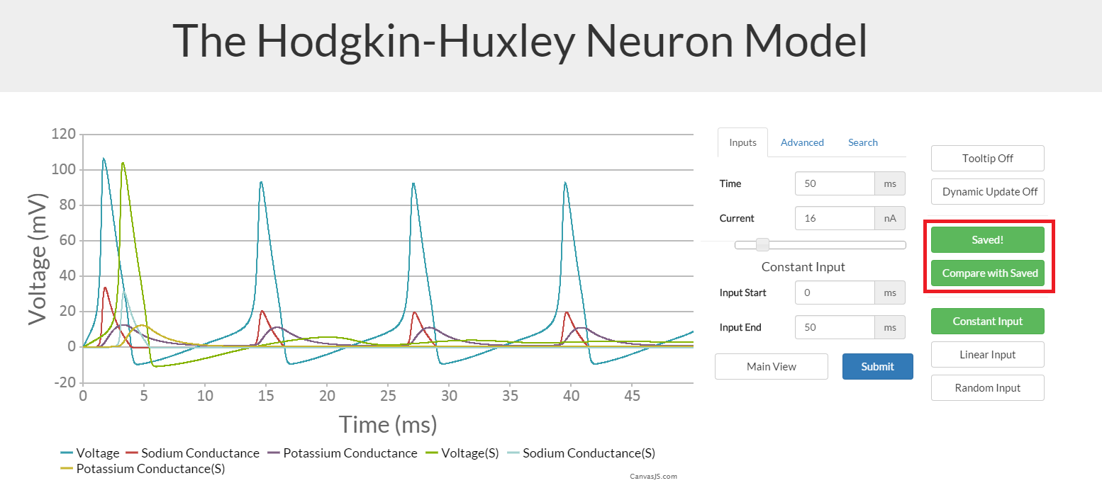
Comparing different inputs
To compare two different sets of input values, first save the first set of values by clicking on the 'Save Current Result' button in the options. Now after inputting the second set of input parameters, click the 'Compare with Saved' button before pressing 'Submit'. This will now show both outputs at once (with different colours). This could potentially be crowded, with up to 6 different data series, so remember to click on the legend to remove unwanted data.
Note that some of the input variables will not change all outputs, for example changing only input current will not neccessarily affect conductance. Also, if comparing two inputs with different lengths of time, the graph will scale to the longer time length.
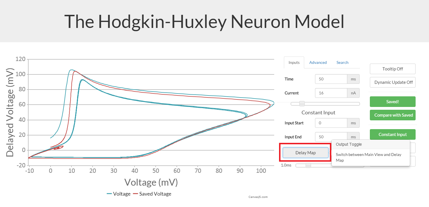
Delay Map
The default type of output simply plots all of the values on a graph. The alternative way of looking at things is using a delay map, which shows the voltage at time t and time t+n, where n can be set by the user. This is useful for looking at the differences and patterns in the output, and especially when comparing uniformity of different outputs.
To select the delay map, either click the 'Toggle output type' box either before submitting a new output, or after the fact. The delay can be changed by using the slider bar under the map.
Neurons
A neuron is a nerve cell, capable of receiving, evaluating, and transmitting information. The process of information transfer is referred to as neuronal signalling. To generate these signals, energy is needed. This energy is in the form of electrical potential across the neuronal membrane, or difference in voltage inside the neuron compared to voltage outside. These voltages depend on the concentrations of potassium, sodium and chloride ions, as well as charged protein molecules inside and outside the cell. The voltage difference across the neuronal membrane in the resting state is typically -70mV (millivolts), which is known as the resting membrane potential. This electrical potential difference means that the neuron has stored energy similar to a battery, and can use it to do work, most importantly signalling. Note that in many neuron models, for the sake of simplicity, the resting state is 0mV.
For a more on neurons, click here.
Action potentials
Neurons have evolved a mechanism to regenerate and pass along signals initiated in the synapse, known as the action potential. The action potential (also known as a spike) is a rapid depolarisation and repolarisation of a small region of the membrane, caused by the opening and closing of ion channels. These voltage-gated ion channels are located in the neuronal membrane at the spike-triggering zone of the axon. When current flows across the spike-triggering zone (when receiving signals), the membrane is depolarised. If the depolarisation is strong enough that a certain threshold is reached, an action potential (or spike) is triggered.
When the threshold is reached, voltage-gated sodium channels open, and sodium flows rapidly into the neuron. This flow of ions further depolarises the neuron, meaning more sodium channels are opened, causing the neuron to be even more depolarised, continuing the cycle (known as the Hodgkin-Huxley cycle). This cycle generates the large depolarisation that is the first portion of the action potential. Next, the voltage-gated potassium channels open, allowing potassium to flow out of the neuron. This outward flow of neurons begins to shift the membrane potential back towards its resting potential.
The opening of the potassium channels outlasts the closing of the sodium channels, causing a repolarising phase of the action potential. This drives the membrane potential further negative than the resting potential. This is known as hyperpolarisation, and causes the potassium channels to close, gradually returning the membrane potential to its resting state. During this time, the sodium channels are unable to open, and another action potential cannot be generated. This is known as a refractory period. This limits the speed of generating action potentials, and ensures that they can only flow in one direction and not self-generate spikes.
For a more on Action potentials, click here.
Neuron Models
A neuron model is a mathematical description of the above properties of nerve cells, and is designed to accurately describe and predict their biological processes. The level of accuracy varies with each model, as many make simplifications in order to improve implementation cost, or focus on specific characteristics. Two of the most common models are the Integrate-and-fire model and the Hodgkin-Huxley model. These models are on the opposite ends of the spectrum in terms of accuracy, where the former is simple but lacking detail, and the latter more complicated but also much more accurate.
For a more on neuron models, click here.
The Integrate-and-fire model explained
In 1907, long before the mechanisms responsible for the generation of neuronal action potentials were known, Lapicque developed a neuron model that is still widely used today
The Integrate-and-fire model is one of the earliest and simplest models of neuron. A neuron is represented by

This is simply the time derivative of the law of capacitance. When the input current(I) is applied, the membrane potential (Vm) increases with time until it reaches a constant threshold, at which point a spike occurs and the voltage is reset to 0. The model then continues to run. The firing frequency thus increases linearly as input current increases.
The model has many variations, each attempting to match real neuron behaviour more closely. One variation is known as the leaky integrate-and-fire model, meaning the problem of time dependent memory is solved by adding a "leak". Without it, if the input stopped, the voltage would stay the same indefinitely, until receiving further input. The leak means the model reflects the diffusion of ions that occurs in the membrane when the threshold is not reached. The equation below shows the updated model, where Rm represents the membrane resistance.

The Hodgkin Huxley model explained
The Hodgkin–Huxley model is a mathematical model that describes how action potentials in neurons are initiated and propagated. This is done using a set of differential equations which approximate the electrical characteristics of excitable cells such as neurons.
This model was developed by Alan Hodgkin and Andrew Huxley in 1952 to explain the initiation and propagation of action potentials in the squid giant axon [2]. It is one of the most successful and widely used models, and was the winner of the Nobel Prize in Physiology in 1963. The model treats each part of the neuron as an electrical element. In the equations below, Vm denotes the membrane potential.

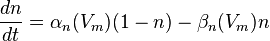
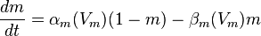

I is the total membrane current per unit area, Cm is the membrane capacitance per unit area. g and V represent the conductance per unit area and reverse potential respectively of sodium (Na), potassium (K), and leak (l). The following equations are also variable, but depend on voltage instead of time.

and are rate constants for each ion channel. n and m are dimensionless quantitates between 0 and 1, that are associated with potassium and sodium channel activation respectively. h is related to sodium channel inactivation.
References
Information taken from Cognitive Neuroscience: The Biology of the Mind, definition quotes from Wikipedia