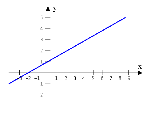
The straight line shown in the graph above can be represented by the linear equation:
y = mx + cwhere c is the y-intercept;
and m is the gradient.
The gradient can be calculated if two points (x1,y1) and (x2,y2) are known:
m = (y2 - y1) / (x2 - x1)
On paper, calculate the value for the gradient and y-intercept, and write the equation for the line.
* Note that the gradient of a line is constant.
Start matlab and open the editor by typing < edit >. Copy this function:
function plot_parabola(x1,x2)
x = linspace(x1,x2);
y = (x.^2)/4;
plot(x,y)
Save the function and run it from the matlab prompt using the values 9.5 and 10.5:
plot_parabola(9.5,10.5)
Estimate the gradient at x = 10 by assuming that the plot is a
straight line with points at
( 9.5 , 22.5 ) and (10.5 , 27.5
).
You can use the same equation as in question 1.
You have just estimated the gradient of the tangent to the curve at x=10.
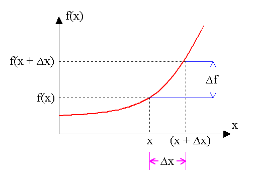
It is possible to create an approximation of a curve using many small straight lines.
The image
below shows two such approximations of parabaloid curves
- note that the
second is a better approximation of a curve than the first.

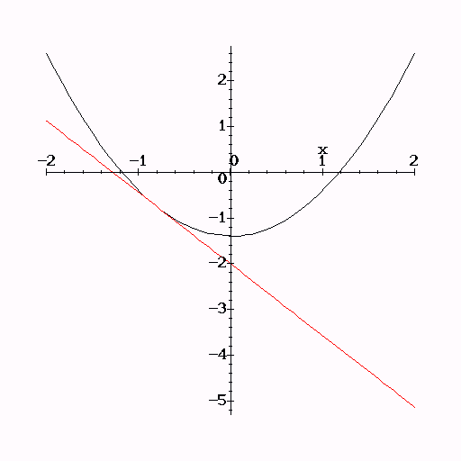
A tangent to a
curve at any given point is the straight line that has the same gradient
as
the curve at that point (the gradient of a curve is constantly changing).
In the graph below the red line is a tangent to the curve at x = -0.8.
Now plot the parabolic curve between -10 and 10:
plot_parabola(-10,10)
You have already estimated the gradient of a tangent to this parabola at x = 10.
Now estimate the gradient of the tangent at x = -10. (The curve is
symmetrical about x=0.)
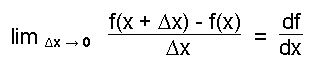
The derivative of a function f at a point x1 is the gradient of the tangent to the curve at x1.
To
approximate the tangent to the curve at point
x1 it is possible to draw a
line through
x1 and
another point x2 and calculate the
gradient of that line.
(NB. a line drawn through two points on a curve is called a secant).

The closer the point x2 is to
x1 and therefore the smaller
x2 - x1 (![]() )
,
)
,
the better the approximation will be.
As ![]() is
made progressively smaller towards the limit value 0 this gives the first derivative of
f.
is
made progressively smaller towards the limit value 0 this gives the first derivative of
f.
.
On paper - use the equation above to calculate the derivative df/dx of the function f(x) = 3x.
Now find df/dx of the function f(x) = x2.
(Remember:
if f(x) = x2 then f(x + ![]() )2
= x2 + 2x
)2
= x2 + 2x![]() +
+
![]() 2)
2)
| if y = x | dy/dx = 1 |
| if y = xa | dy/dx = axa-1 |
| if y = sin(x) | dy/dx = cos(x) |
| if y = cos(x) | dy/dx = -sin(x) |
Use the < linspace > function to create an array of 100 equally spaced values between -10 and 10.
Plot the curve y = x3. On the same axes plot the derivative of the curve dy/dx in a different colour.
In a new < figure > plot the curve y = sin(x). On the same axes plot the derivative in a different colour.