Discrete Dynamics Lab

Update Sept 2015 ddlabz03 New options: density plot t0 -> t1 -- 1-pixel jump-graph nodes -- 3d neighborhoods -- classifying rule-space patch options -- 2d networks patch options -- cell division colors -- dynamic trace on-the-fly Supersedes DDLabx11, May 2013 and includes updates since the publication of Exploring Discrete Dynamics in May 2011. Download ddlabz03 for Linux, Mac, Cygwin and DOS. The ddlabz03 source code is available, including Makefiles, readme, GNU license, and notes.

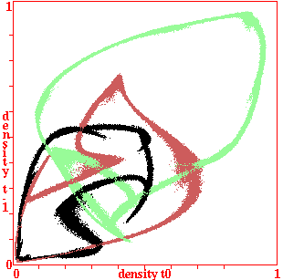
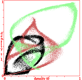
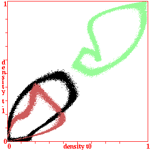
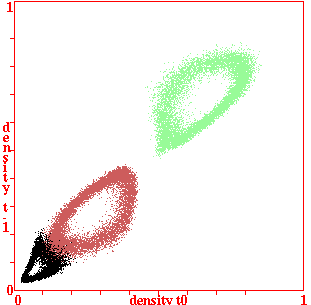
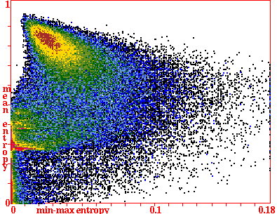
density plot x:t0 -> y:t1, v3k6, 2d 222x222 kcode=(hex) 020282815a0254, index=4, fully random wiring

DDLab has been updated at regular intervals since its release in 1995. Its precursor was the Atlas software included on diskette inside the back cover of "The Global Dynamics of Cellular Automata". For a list and download of this and older versions click here. Below are links to previous updates, May 2013 xxJan 2013 xxxxJune 2012 xxxxxxNov 2005 xxxxxxxxDec 2003 xxxxxxxxxxJuly 2001 xxxxxxxxxxxxFeb 1999 xxxxxxxxxxxxxxSept 1997

Some of the Sept 2015 updates are summarised below. Click figures to enlarge.
EDD #x.x.x refers to the relevant section in "Exploring Discrete Dynamics". All updates since May 2011 will be included in the 2nd edition of EDD, under preparation.

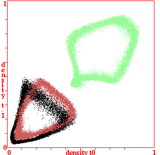
density plot x:t0 -> y:t1 examples

A new on-the-fly option is a density plot where the value density at t0 (x-axis) is plotted against the value density at t1 (y-axis). This can be interesting when the densities follow a periodic oscillation, which occurs for complex rules with random wiring. Complex rules are those with emergent glider interactions or large scale pattern dynamics. Collections of complex rules are available with DDlab, as described in EDD #3.7.1. The 4 examples on the left relate to k-totalistic rules, v3k6, 2d 66x66, with fully random wiring, where 0=green 1=red 2=black. The kcodes are from the complex rule sample index 4, 30, 42 and 52. To replicate these results, entropy-density must be active while running space-time patterns. Then toggle the density plot in a separate window with on-the-fly key ";" (semi-colon). Key g changes to a random rule in the complex rule sample. For consecutive indexes, interupt with q, enter G then 1. The random wiring can be toggled to local wiring with key 7.

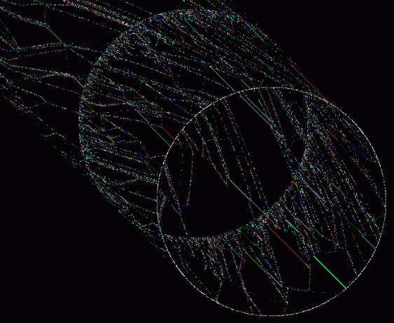
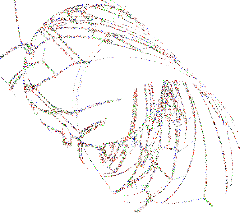
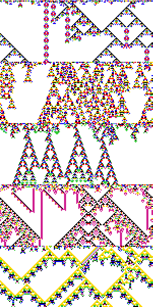
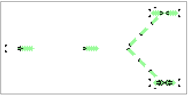
1-pixel jump-graph nodes -- for a big 1d scrolling tube

The nodes of the network-graph (EDD chapter 20) can now be reduced to one pixel. This allows large system sizes for the 1d scrolling tube, 60000+. The examples are snapshots of scrolling tubes for ECA rule 110 (filtered) showing interacting gliders, with time-steps shown every "skip" iterations to increase the glider angle. The white background example has 2000 cells and one random initial state visible ("skip"=10). The black background example has 10000 cells and two random initial states visible one of which was set at the present moment ("skip"=20). The present moment is at the front of the scrolling tube, with the past history scrolling towards the back. For applications, see Computing with virtual cellular automata collider Martinez, G.J. ; Adamatzky, A. ; Mclntosh, H.V.

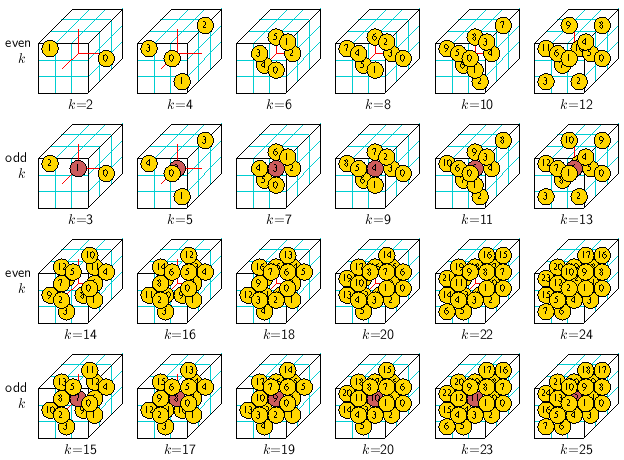
3d neighborhoods revised

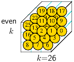
All the 3d neighborhoods are now contained within a 3x3x3 cube, and have been extended to k=27 and somewhat modified to those defined in the first edition of EDD. The figures on the left and above show how 3d neighborhood templates are defined and indexing in ddlabz03, for k=2 to 27. k=1 is self evident. For even k the target cell itself is not included in the neighborhood. The view is isometric as if looking up into a cage. The placement of the neighborhood within the cube is chosen to achieve maximum symmetry, though there would be alternative choices which could be reprogrammed.

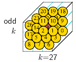
3d neighborhoods presenterd in 2d

The 3d neighborhood templates are simultaniously displayed in 2d as well as 3d. These 2d graphics for k=2 to 27 show the 3 levels of each 3x3x3 cube, one below the other, representing the neighborhood templates. The index numbers start with 0 then from right to left in ascending rows. The index numbering can be toggled on/off i.

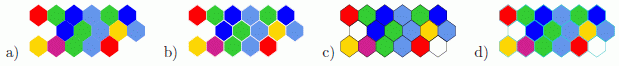
classifying rule-space 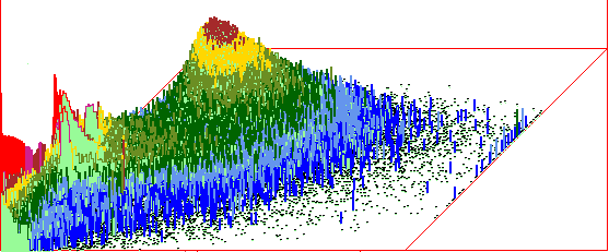scatter plot histogram the scatter plot, which can be probed with the mouse

patch options listing rules in the patch scanning rules in the patch last 5 rules from the list above

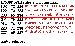
Figures on the far left show an example scatter plot for classifying rule space (described in EDD chapter 33, v8k3B50.sta). There are many methods for sorting, probing, listing, saving, and displaying the rules in these plots, but some new methods and options have been added, notably defining a "patch" by 2 successive right mouse clicks anywhere on the scatter plot, the following reminder is shown. xxxxselect rules - point-click mouse button: probe-left, patch-right After the second right mouse click, a prompt to activate the patch appears, xxxxpatch: x2=237 y2=66, activate-p Once activated with p, the coordinates of the patch can be amended or accepted, xxxxpatch coords (def 226 75 237 66) keyboard-k accept-def: If the patch is active, after the scatter plot is reloaded, patch-p appears in the prompt in EDD #33.5, xxxxlist: all-l patch-p coords-c, sort-s backtrack-q (sublist-S save-SS) xxxx--(S/SS see note below) Enter p to list the rules in the patch. A useful way to see space-time patterns for the different rules in the patch is to scan in automatic blocks of time-steps -- enter V on-the-fly giving the following prompt. xxxxrule sample: load new-n, rule index/scan 1-176398 (198-def): Enter return to accept, giving the following, xxxxscan time-blocks from index 198: incr-i keep-k no-blocks-def: Then enter i to change rules (k keeps the same rule changing random seeds). The sample index increases for eack next block, but stays within the rule patch, recycling to the patch start index. The next prompt allows the block time-steps to be revised, set here to 60. xxxxset time-block (def 150): Then define the initial state, here set to all random (def), xxxxseedtype: block-v single-5/6 (def-all): This method was used to search the scatter plot for The X-rule: universal computation in a non-isotropic Life-like Cellular Automaton Jose Manuel Gomez Soto, Andrew Wuensche Note: "sublist-S and save-SS" are special functions to create a scatter plot from a list of rules inserted within the source code.

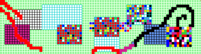
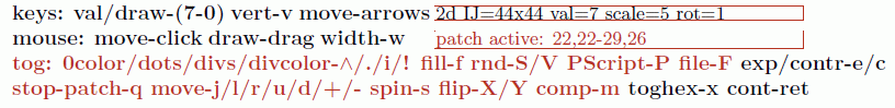
2d networks -- patch options playing with a 2d 10x8 active patch in an 8 value 2d seed 88x22 options in red apply to the patch only -- deactivate with stop-patch-q

New options have been added for editing 2d networks. In particular a patch of any size can be defined by the last two left mouse clicks, and activated with patch-p in EDD prompt #21.4. Thereafter most editing options, colored red in the prompt as illustrated, apply only to the patch rather than to the whole network. For example the patch can be independently moved, jumped/copied to any cursor position, flipped, spun, complimented, and division colors changed. The patch can be filled with colors/values or random patterns. Drawing with the mouse cursor or keyboard still applies to the whole network as well the patch. The patch can be saved/loaded as an *.eed file, or saved as a *.ps PostScript image. These features have been added in order to make it easier to design, edit and test spacial patterns for rules such as the game-of-Life, the spiral-rule, and the X-rule, in order to create desired particle collisions, gliders, static structures, glider-guns, and combinations to implement logical gates for universal computation.. These method were used to design configurations for The X-rule: universal computation in a non-isotropic Life-like Cellular Automaton Jose Manuel Gomez Soto, Andrew Wuensche

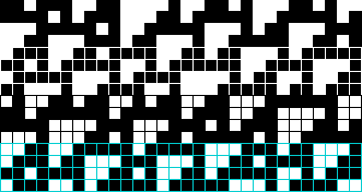
cell division colors: none-white-black-lightblue on-the-fly 1d on-the-fly 2d (hex), and setting a seed

There are new options for division lines between cells, and division line color, which apply on-the-fly while space-time patterns are running (EDD #32.9.3), or at the seed prompt for 1d or 2d (EDD #21.4, above). Enter on-the-fly key hits, or at the seed prompt, as follows, i --- to toggle divisions on-off. ! --- for a 3-way toggle of the division color -- white, black, and light blue.

"dynamic trace" on-the-fly option

A new on-the-fly "dynamic trace" option shows dynamic time-trails against a zero background. To show the dynamic trace enter h on-the-fly to toggle/cycle through five ways of displaying space-time patterns, including "frozen" and "frequency" (EDD #32.11). Dynamic trace is the first way, and is the most effective to show the path of gliders in 2d, but also works in 1d and 3d. The length of the trace is adjustable (enter H, EDD #32.11.2), in this example the "generation size"=20 time-steps. 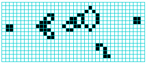This example shows two glider-guns and a collision making a new glider, from The X-rule: universal computation in a non-isotropic Life-like Cellular Automaton Jose Manuel Gomez Soto, Andrew Wuensche

the bare attractor -- limit backward steps to zero East Game-of-Life glider-gun attractor

A new option generates a "bare" attractor -- without any incoming transients. For single basins the number of backward steps can be set to zero -- enter 0 at the prompt in EDD #29.5. Because the data is derived from forward itteration, reverse algorithms do not come into play -- the graphic image of attractors for very large networks, including 2d, can be generated. The figure on the left is Gosper's glider-gun from the game-of-Life within a 38x16 lattice, shown as an attractor with period 30. Below is the initial state, located just below the state marked East in the attractor cycle. Note the eater positioned to destroy emergent gliders. Game-of-Life glider-gun snapshot

Return to the Discrete Dynamics Lab home page.
Last modified: Sept 2015