Research Methods 1: Statistics
Problem-Sheet 6: Dependent-Means t-tests:
1. Ten subjects take a test
of motor coordination, once after drinking a pint of beer and once without
drinking alcohol. Their times in seconds to complete the task were:
|
Subject: |
With beer: |
Without beer: |
|
1 |
12.4 |
10.0 |
|
2 |
15.5 |
14.2 |
|
3 |
17.9 |
18.0 |
|
4 |
9.7 |
10.1 |
|
5 |
19.6 |
14.2 |
|
6 |
16.5 |
12.1 |
|
7 |
15.1 |
15.1 |
|
8 |
16.3 |
12.4 |
|
9 |
13.3 |
12.7 |
|
10 |
11.6 |
13.1 |
Perform a matched-pairs (also
known as a dependent-means) t-test to test whether drinking beer makes you
slower at the task. [Answer: t = 2.18, p>0.05]. How would you design this
experiment, in order to ensure a fair result?
2. An experiment is performed
to see if motorcycling makes people happier. Ten individuals are given a
happiness questionnaire before and after 30 minutes' motorcycle riding. The
scores are shown below (high score = high degree of happiness).
|
Subject: |
Before: |
After: |
|
1 |
5 |
7 |
|
2 |
4 |
8 |
|
3 |
6 |
9 |
|
4 |
4 |
10 |
|
5 |
7 |
11 |
|
6 |
3 |
3 |
|
7 |
4 |
5 |
|
8 |
6 |
5 |
|
9 |
3 |
3 |
|
10 |
5 |
5 |
(a) Calculate the mean and
standard deviation for each condition. (Use the s.d. formula which gives the s.d.
as an estimate of the population s.d.). [Answers: 4.7 and 1.34; 6.6 and 2.84].
(b) Perform a dependent-means
t-test. [Answer: t = 2.63, p<0.05].
What problems are there in
performing this experiment, in practice? (Apart from difficulty in persuading the
individuals concerned to stop riding the bikes!)
3. Five articles are selected
randomly from each of twelve "Daily Stir" journalists. The mean
number of lies and libellous comments per article is recorded for each
journalist. These journalists are then sent on a creative writing course, after
which five of their more recent articles are selected at random and analysed as
before. Here are the data:
|
journalist: |
1 |
2 |
3 |
4 |
5 |
6 |
7 |
8 |
9 |
10 |
11 |
12 |
|
no. of lies before course: |
3 |
9 |
16 |
5 |
6 |
10 |
12 |
11 |
6 |
9 |
2 |
6 |
|
no. of lies after course: |
5 |
8 |
42 |
7 |
12 |
12 |
10 |
14 |
7 |
11 |
5 |
6 |
(a) What are the mean and
standard deviation for each condition? [Answers: 7.92 and 4.01; 11.58 and
10.03].
(b) Perform a matched-pairs
t-test on these data. [Answer: t = 1.73,
p>.10].
(c) Journalist number three
gets a new job at the Daily Moron, on the strength of his outstanding
performance following the creative writing course. Reanalyse the data, omitting
this subject. [Answers: mean and standard deviation for "before"
condition are 7.18 and 3.25; mean and s.d. for "after" condition are
8.82 and 3.12; t = 2.52, p<0.05].
4. An experiment is performed
to determine which is more unpleasant: singing by Kylie Minogue or singing by
Jason Donovan. Subjects are manacled to a chair, and forced to listen to either
a Kylie song and then a Jason song, or vice versa. The dependent variable is
the time (in seconds) before the first scream is uttered. Which singer is considered
more unpleasant, Jason or Kylie? Here are the data (presented in this way for
clarity: subjects 1 to 7 heard Jason before Kylie, while subjects 8 to 14
suffered Kylie before Jason). Calculate the mean and standard deviation for
each condition, and perform a dependent-means t-test on the data. [Answer: mean
and s.d. for Kylie condition = 4.42 and 2.62; mean and s.d. for Jason condition
= 4.71 and 3.12; t = 0.56, p>.50].
|
subject number: |
1 |
2 |
3 |
4 |
5 |
6 |
7 |
8 |
9 |
10 |
11 |
12 |
13 |
14 |
|
Kylie song: |
6 |
4 |
7 |
2 |
1 |
8 |
2 |
3 |
1 |
3 |
4 |
5 |
9 |
7 |
|
Jason song: |
8 |
3 |
3 |
1 |
1 |
9 |
3 |
2 |
3 |
6 |
3 |
7 |
11 |
6 |
First-Year Research Methods: Worked
Solutions to Problem Sheet 6:
Question
1:
(a) Work out the difference score (D) for each subject:
|
|
with beer: |
without beer: |
difference (D): |
|
subject 1: |
12.4 |
10.0 |
2.4 |
|
subject 2: |
15.5 |
14.2 |
1.3 |
|
subject 3: |
17.9 |
18.0 |
-0.1 |
|
subject 4: |
9.7 |
10.1 |
-0.4 |
|
subject 5: |
19.6 |
14.2 |
5.4 |
|
subject 6: |
16.5 |
12.1 |
4.4 |
|
subject 7: |
15.1 |
15.1 |
0.0 |
|
subject 8: |
16.3 |
12.4 |
3.9 |
|
subject 9: |
13.3 |
12.7 |
0.6 |
|
subject 10: |
11.6 |
13.1 |
-1.5 |
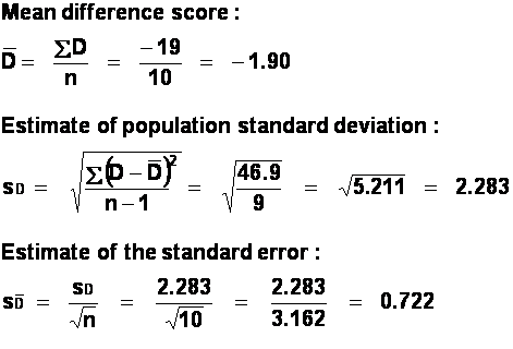
(b) Find SD,
the sum of the difference scores: SD = 16.0.
Divide SD by n (the number of difference scores) to get the mean
difference score, ![]() .
.
(c) Find the standard deviation of the difference scores.
Here is the formula. (Don't get confused by the terminology here.
"S.D." or "s.d." are abbreviations in English for "standard deviation". The mathematical symbol for the sample
standard deviation is "s", and "sD" in this
context stands for "standard deviation of the Difference
scores"!)

This
standard deviation is a measure of the spread of the difference scores around
the mean difference score. If this s.d. is large, it means that difference
scores varied widely - so that some subjects might show a large difference
between the two conditions that they participated in, while others might show a
small difference; and/or it might reflect a difference in the opposite
direction (i.e., with some subjects performing better on the second test than
on the first, and others performing better on the first test than on the last.
This seems to be the case in our experiment, as shown by the fact that some
differences are negative in sign while others are positive).
(d) Find the standard error of the mean of the difference
scores. This is simply the standard deviation of the difference scores, divided
by the square root of the number of difference scores:

(Again, it's easy to get confused by the notation here:
the standard error is designated by S followed by a D with a bar over the top, whereas
the standard deviation has the same symbols but without the little bar. The SD (without a little bar) within this equation
stands for the whole of the standard deviation equation in section (c) above).
(e) Finally, find t. To get t, take the mean difference score (the result of
step b), and divide it by the standard error of the mean of the difference
scores (the result of step d).
This gives t = 2.18.
The degrees of freedom are given by the number of difference scores minus one;
in this case, d.f. = 10-1 = 9 degrees of freedom. Consulting a table of
critical t-values, we find that the critical t at the p = 0.05 significance
level for a two-tailed test is 2.262. Our obtained t is smaller than this;
hence we conclude that it is not statistically significant. In other words,
there is no reason to reject the null hypothesis, that the difference between
our two conditions is due merely to chance (i.e., that what we effectively have
is two samples from the same "population", which differ merely due to
random sampling variation).
How would you design this experiment, in order to ensure
a fair result? You would have to take care to avoid order effects, which are
always a potential problem with repeated measures designs. You would have to
make sure that half of the subjects did the two conditions in one order, and
the other half did the conditions in the opposite order; and that you allowed
enough time between tests for the effects of the beer to wear off, for those
people who experienced this condition first!
Question
2:
|
|
before: |
after: |
difference (D): |
|
subject 1: |
5 |
7 |
-2 |
|
subject 2: |
4 |
8 |
-4 |
|
subject 3: |
6 |
9 |
-3 |
|
subject 4: |
4 |
10 |
-6 |
|
subject 5: |
7 |
11 |
-4 |
|
subject 6: |
3 |
3 |
0 |
|
subject 7: |
4 |
5 |
-1 |
|
subject 8: |
6 |
5 |
1 |
|
subject 9: |
3 |
3 |
0 |
|
subject 10: |
5 |
5 |
0 |
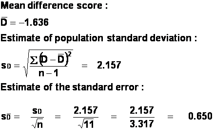
Just looking at the difference scores, we can see that
most subjects were happier after riding the motorcycle than they were before. Three
subjects showed no difference, and one subject was happier before the ride than
after.


We have ten difference scores, so
d.f. = 10 - 1 = 9.
Comparing our obtained t, -2.63, to the critical t for a 0.05 significance level with a
two-tailed test (2.262), we find that our obtained t is larger. (Ignore the
sign when comparing them: the absolute value of t is 2.63, which is bigger than
2.262). Therefore we reject the null hypothesis and conclude that our two
conditions differ as a consequence of what we did to the subjects (i.e., the
motorcycle ride). In other words, the difference between our sample means is so
big that it is unlikely to have occurred merely by chance.
However, in practice there would be problems in
interpreting this result as showing that "motorcycle riding makes people
happier". All of our subjects were tested in the same order, i.e. first
before riding and secondly after riding. Consequently, we have not eliminated
other possible causes for our observed results. It might be, for example, that
people tested twice on a happiness questionnaire usually score higher on the
second test - regardless of any experimental manipulation we might choose to
insert between tests. If this were true, the motorcycle ride might have nothing
to do with our results at all. This is an important point: a statistics test
performed correctly on data from a badly-designed experiment may give you a
plausible result which is nevertheless actually worthless in terms of the
conclusions which you can validly draw from it. What would be a better design
in this particular case? We have the problem that we cannot run half of our
subjects in the opposite order - you cannot undo a motorcycle ride! We could
assign subjects randomly to two groups, an experimental group (who get a
motorcycle ride) and a control group (who do not). Then, we could compare the
happiness scores of the two groups, using an independent-means t-test.
Question
3:
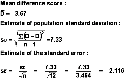
(b)
|
journalist: |
1 |
2 |
3 |
4 |
5 |
6 |
7 |
8 |
9 |
10 |
11 |
12 |
|
lies before course: |
3 |
9 |
16 |
5 |
6 |
10 |
12 |
11 |
6 |
9 |
2 |
6 |
|
lies after course: |
5 |
8 |
42 |
7 |
12 |
12 |
10 |
14 |
7 |
11 |
5 |
6 |
|
difference (D): |
-2 |
1 |
-26 |
-2 |
-6 |
-2 |
2 |
-3 |
-1 |
-2 |
-3 |
0 |


There are (12-1) = 11 degrees of freedom.
The critical value of t (obtained from a table of t-values)
for 11 d.f. is 2.201, for a two-tailed test and a 0.05 significance level. Our
obtained t is smaller than this value, and so we cannot reject the null
hypothesis, that there is no difference between the number of lies produced by
these writers before and after their creative writing course. (Note that, even
if there were, we would have problems attributing the change to the creative
writing course because of the uncontrolled order problems, as in the previous
question).
(c) Reanalysing the data, with journalist number three
omitted (and the remaining journalists renumbered accordingly):
|
journalist: |
1 |
2 |
3 |
4 |
5 |
6 |
7 |
8 |
9 |
10 |
11 |
|
lies before course: |
3 |
9 |
5 |
6 |
10 |
12 |
11 |
6 |
9 |
2 |
6 |
|
lies after course: |
5 |
8 |
7 |
12 |
12 |
10 |
14 |
7 |
11 |
5 |
6 |
|
difference (D): |
-2 |
1 |
-2 |
-6 |
-2 |
2 |
-3 |
-1 |
-2 |
-3 |
0 |


t = -2.52, with
(11-1) = 10 degrees of freedom. Our obtained t value is larger than the
critical value of t for a two-tailed test (2.228). we can reject the null
hypothesis, that there is no difference in the number of lies produced by the
journalists in the two conditions (i.e., before and after the creative writing
course), in favour of the alternative hypothesis that there is a difference.
However, we are still faced with the problem of interpreting these results
because of the problems with the experiment's design. The solution would be to
use an independent-measures design: randomly allocate journalists to one of two
groups, journalist who took a creative writing course and journalists who did
not. Their subsequent capacities for lying could then be compared with an
independent-means t-test.
Question
4:
|
subject no.: |
1 |
2 |
3 |
4 |
5 |
6 |
7 |
8 |
9 |
10 |
11 |
12 |
13 |
14 |
|
Kylie song: |
6 |
4 |
7 |
2 |
1 |
8 |
2 |
3 |
1 |
3 |
4 |
5 |
9 |
7 |
|
Jason song: |
8 |
3 |
3 |
1 |
1 |
9 |
3 |
2 |
3 |
6 |
3 |
7 |
11 |
6 |
|
D: |
-2 |
1 |
4 |
1 |
0 |
-1 |
-1 |
1 |
-2 |
-3 |
1 |
-2 |
-2 |
1 |
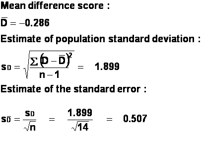
Just looking at the difference scores, we can tell
that there is not much difference between these two conditions: the differences
are small, and about half of the subjects thought Kylie was worse than Jason
while the other half thought the opposite.


There are (14-1) = 13 d.f.
The critical t-value is 2.160 for a two-tailed test. Our obtained
t of -0.56 is much smaller than this, and so we have no reason to reject the
null hypothesis that there is no difference between the two singers - both
cause people to scream very quickly!
[N.B. In all these examples, our t-values are negative. This
is just a coincidence: had we ordered our two data columns the opposite way
round, then we would have obtained positive t-values. In comparing obtained and
critical t-values, ignore the sign of the obtained t when doing a two-tailed
test].