Research Methods 1: Problem Sheet 4:
1. The following data are scores on two tests of visual imagery (each pair of scores represents the scores obtained from one subject).
Imagery test 1: 10 14 15 26 34 38 40 45 47 50 55 60 61.
Imagery test 2: 5 2 11 9 16 18 12 30 50 85 86 89 83
(a) Draw a scatterplot of these data.
(b) calculate a Pearson's correlation coefficient for these scores. [Answer: 0.87].
(c) Calculate a Spearman's correlation coefficient for these scores. [Answer: 0.94].
(d) Explain, in words, why in this particular example the Spearman's correlation coefficient is higher than the Pearson's correlation coefficient.
2. A child psychologist gives a reading test to 200 5-year olds. The scores are normally distributed, with a mean of 70 and a standard deviation of 10.
(a). How many children have a reading score of 80 or above?
(b) What proportion of children have a reading score between 67 and 73?
(c) The psychologist decides that all children whose reading score is more than one standard deviation below the mean will receive remedial treatment. How many of the children in her sample will get remedial treatment?
(d) How many children have a reading score between 36 and 55?
3. The following data represent scores on a maths test:
15 7 23 19 4 10 13 17 2 30 14 17 22 15 12 18 4 18 13 21
(a) Calculate the mean and standard deviation of these scores. [Answers: mean = 14.7; s.d. = 6.83].
(b) If these data were normally distributed, what proportion of the scores would you expect to be within one standard deviation of the mean? [Answer: 68%].
(c) What proportion of these scores are in fact within one standard deviation of the mean? [Answer: 70%].
4. IQ scores are normally distributed with a mean of 100, and a standard deviation of 15.
(a) What proportion of the population would have an IQ less than 76? [Answer: 0.0548].
(b) What proportion of the population would have an IQ between 96 and 120? [Answer: 0.5146].
(c) What proportion of the population would have an IQ less than 124? [Answer: 0.9542].
(d) What proportion of the population would have an IQ above 83? [Answer: 0.8706].
(e) Below which IQ score do 76% of the population fall? [Answer: 110.59].
(f) Above which IQ score do 15% of the population fall? [Answer: 115.46].
(g) Above which IQ score do 60% of the population fall? [Answer: 96.20].
(h) Between which IQ scores do the central 20% of the population fall? [Answer: 96.20 to 103.80].
(i) Between which IQ scores do the central 90% of the population fall? [Answer: 75.33 to 124.68].
5. (a) Yamahondukuzikawa car manufacturers incorporated are concerned about the productivity of some of the workers in their new Welsh production plant. The average output of their workers overall is 20 fully-assembled cars per day per worker, with a standard deviation of six. However, they have measured the productivity of a sample of 35 randomly-chosen employees, and are shocked to discover that workers in this sample are managing to produce only 18 cars per day per worker. Mr. Yamahondukuzikawa suspects this is due to these particular workers' extended breaks for leeks: is he justified in his assumption that these workers are lazy, or could the difference between 18 and 20 be attributable to sampling variation? With a sample size of 35, what is the probability of obtaining a sample mean of 18 or less from this population? Is Mr. Yamahondukuzikawa being over-hasty in ordering hara-kiri for these workers? [Answer: z = -1.972. The probability of obtaining a sample mean of 18 or lower is 0.0244].
Hint: this is a z-score problem, like question 4. However, in question 4 you are comparing a single score to the population of scores from which it is derived. In this problem, you are comparing a sample mean (from a sample with an N of 35) to a population for which you know the mean and standard deviation. What you want to know is how often a sample mean of 18 or less would be obtained by chance. The z score formula in this case is:

"standard error" population standard deviation
![]()
![]()
![]()

(b) Yamahondukuzikawa inc. execute these 35 workers as an example to the rest. A year later, they review the productivity of the Welsh workers. They take another random sample, this time of 10 workers (since the rest are all cowering in the toilets), and once again find that each worker is producing only 18 cars per day. The overall productivity of the factory remains the same, at 20 cars per worker with an s.d. of 6. How often would a sample mean of 18 or less be obtained with a sample size of 10? What should the company do this time? [Answer: z = -1.054. The probability of obtaining a sample mean of 18 or less is 0.1469].
Research Methods 1: Worked Solutions to Problem Sheet 4:
Question 1:
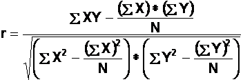
(b). To calculate the Pearson's correlation coefficient, "r", we can use the following formula:


1(c). To calculate the Spearman's correlation coefficient, "rho", we can use the following formula:

Call one variable "X" and the other variable "Y". (It doesn't matter which imagery test you call "X", as long as you are consistent with your labelling throughout the rest of the calculations). Here, the imagery test 1 scores will be used as the X scores, and the imagery test 2 scores will be used as the Y scores.
First, rank the data for each variable in turn (lowest number is given a rank of 1, next is given a rank of 2, etc.).
Second, find the values of "D". These are obtained by subtracting each Y-rank from its corresponding X-rank.
Third, find the values of "D2". These are obtained by squaring each of the D-values.
The results of all these
calculations are shown in the following table:
|
X value |
10 |
14 |
15 |
26 |
34 |
38 |
40 |
45 |
47 |
50 |
55 |
60 |
61 |
|
X rank |
1 |
2 |
3 |
4 |
5 |
6 |
7 |
8 |
9 |
10 |
11 |
12 |
13 |
|
Y value |
5 |
2 |
11 |
9 |
16 |
18 |
12 |
30 |
50 |
85 |
86 |
89 |
83 |
|
Y rank |
2 |
1 |
4 |
3 |
6 |
7 |
5 |
8 |
9 |
11 |
12 |
13 |
10 |
|
D |
-1 |
1 |
-1 |
1 |
-1 |
-1 |
2 |
0 |
0 |
-1 |
-1 |
-1 |
3 |
|
D2 |
1 |
1 |
1 |
1 |
1 |
1 |
4 |
0 |
0 |
1 |
1 |
1 |
9 |
Fourth, add up all of the D2 values, to get SD2. SD2 = 22.

1 (d). Spearman's correlation coefficient is a measure of the amount of "monotonic" relationship between two variables: i.e., the extent to which one variable increases as the other one increases, regardless of the numerical size of the increase*. Because the data for each variable are ranked, it addresses the question "do subjects who rank highly on one variable also rank highly on the other, and vice versa?" In contrast, Pearson's correlation coefficient is a measure of the linear relationship between two variables: if one increases by a certain amount, does the other variable also increase by a comparable amount? In our example, the data are clearly related, as shown by the scatterplot: as scores increase on test 1, they also increase on test 2. However, the relationship is curvilinear, rather than linear: as values on test 1 increase, values on test 2 increase slowly when the corresponding test 1 value is low, but rapidly when the test 1 value is high. This does not affect the Spearman's correlation coefficient because Spearman's rho does not take the numerical values of the scores into account. However it does affect the Pearson's correlation, leading to an underestimation of the strength of the relationship between the two variables when Pearson's r is used. This is why you should always draw at least a rough scatterplot to see what your data look like, before performing a correlation test.
* (For simplicity's sake, I've only talked about positive correlations in this paragraph - where, as values on one variable increase, so too do values on the other variable. Of course, exactly the same arguments apply to negative correlations - where, as values on one variable increase, values on the other variable decrease).
Question 2:
These are all "z-score" problems. It usually helps to do a rough graph of each problem, so that you can see what area under the normal curve needs to be found.
2(a) How many children have a reading score of 80 or more?
X = 70 X=80 s.d. = 10 N = 200![]()
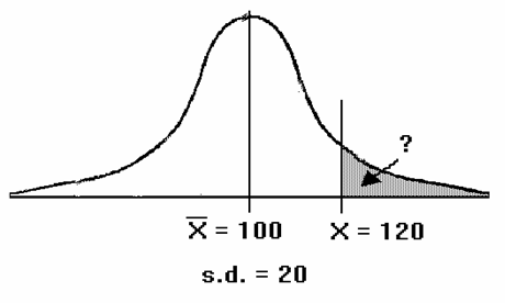
Find the shaded area, by converting X into a z-score and then using the "area under the normal curve" table.

The table tells us that the "area beyond z", for z = 1.000, is 0.1587.
The number of children with a reading score of 80 or above, is 0.1587 * 200 = 31.74 (32 children!).
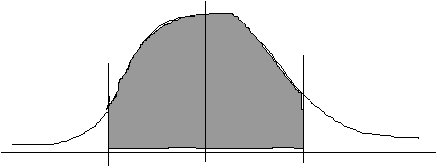
2(b) What proportion of children have a reading score between 67 and 73?
![]()
67 and 73 are the same distance from the mean; therefore we need only work out one area (e.g., the area between the mean and 73) and then double it, since the z-scores (and hence areas under the curve) corresponding to 67 and 73 would be identical.

The "area between the mean and z" for 0.3000 is 0.1179.
Therefore, 2* 0.1179 = 0.2358 of the children would be expected to have scores between 67 and 73 (in other words, 23.58% of 200, or 47 children).
2(c) How many children get remedial treatment?


![]()
Ignore the sign: look up the "area beyond z" for 1.000. This is 0.1587.
0.1587 * 200 = 31.74 (= 32!) children will get remedial treatment.
2(d) How many children have a reading score between 36 and 55?
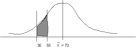
First, find the "area between the mean and z" for the raw score of 36.
![]()
The area under the curve which corresponds to this z-score is 0.4997.
![]()
The area under the curve which corresponds to this z-score is 0.4332.
Third, find the difference between these two areas, because this gives us the area that we actually want. 0.4997 - 0.4332 = 0.0665. In other words, 6.65% of the children (13 kids) have scores between 36 and 55.
Question 3:
3(c) To find out how many scores are within one standard deviation of the mean, we simply count up how many scores fall between 7.87 (= 14.7 - 6.83) and 21.53 ( = 14.7 + 6.83). Thirteen scores (15, 19, 10, 13, 17, 14, 17, 15, 12, 18, 18, 13 and 21) fall between these limits. (13/20)*100 = 65% of scores fall within one standard deviation either side of the mean.
Question 4:
Again, these are all z-score problems, which it's best to graph first.
![]() 4(a)
4(a)


![]()
The "area beyond z" for 1.600 is 0.0548. In other words, 5.48% of the population have IQ's of 76 or less.
![]() 4(b)
4(b)
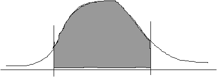
![]()
First, find the area between 96 and 100.
![]()
The "area between the mean and z" = 0.1064.
Secondly, find the area between 120 and 100.
![]()
The "area between the mean and z" = 0.4082.
Finally, add these areas together: 0.1064 + 0.4082 = 0.5146 = 51.46% of people have IQ's between 96 and 120.
4(c)
100
124
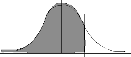
We know that .5000 of the area under the curve (corresponding to half of the total number of scores) falls below 100. Therefore we just have to find the "area between the mean and z" for 124 and then add .50 to it.
![]()
The area between the mean and z is 0.4452.
0.4452 + .5000 = 0.9452. In other words, 94.52% of the population would be expected to have IQ's of 124 or less.
![]()
 4(d)
4(d)
83
124

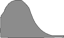
Find the z-score for 83 ( = -1.133); find the "area between the mean and z" ( = 0.3708); add the area above the mean ( = 0.500). 87.08% of people would be expected to have IQ's of 83 or above.
![]()
4(e)
100
X = ?
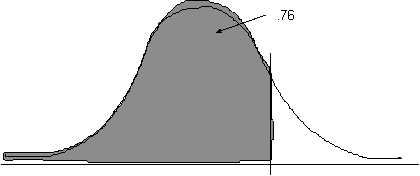
Here, we know the know the area (0.7600); we want to know what raw score cuts off this region.
Use the formula which converts a z-score into a raw score: X = m + z s .
X = 100 + (0.71 * 15)
X = 110.65.
76% of the population would be expected to have an IQ of 110.65 or less.

4(f)

X = ?
X = m + z s .
X = 100 + (1.03 * 15)
X = 115.45
15% of the population would be expected to have an IQ of 115.45 or more.
4(g)

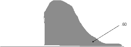
X = ?
X = m - z s . (Minus, because X falls below the mean).
X = 100 - (0.26 * 15)
X = 96.10 (or 96.20 if you used a z of 0.25).
In other words, 60% of people would be expected to have IQ's of 96.1 or above.
![]()
![]()

![]()
 4(h)
4(h)
X = ?
X = ?
![]()
Here, it's the "central 20%" that we are concerned with. In other words, find the z corresponding to an "area between the mean and z" of 0.10. (z = 0.25 or 0.26, depending on whether you use 0.1026 or 0.987 as your "area").
X = m + (0.25 * 15) = 103.75.
X = m - (0.25 * 15) = 96.25.
In other words, 20% of the population would be expected to have IQ's between 96.25 and 103.75.
![]()
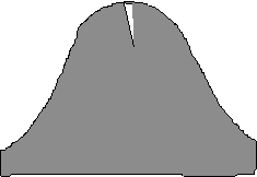 4(i)
4(i)

90% = .90 =.45 either side of the mean. Therefore we need to find the z-score which corresponds to an "area between the mean and z" of 0.45. z = 1.65.
X = m + (1.65 * 15) = 124.75.
X = m - (1.65 * 15) = 75.25.
90% of the population would be expected to have IQ's between 75 and 125. (Note the rounding errors due to using 1.65 rather than 1.64 as a z-score).
Question 5:
5(a) We know that the population has a mean of 20 and a standard deviation of 6; and we have a sample mean of 18. The sample size is 35. We want to know how often we would be likely, by chance, to obtain a sample mean this small or smaller. It helps to do a rough graph of the problem:
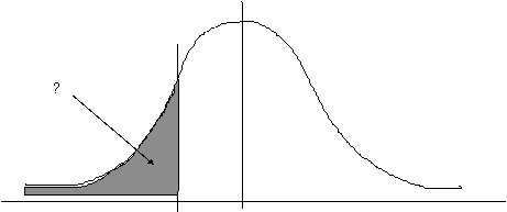

Basically, we want to know what the relationship is between our sample mean, and our population. z-scores are the key to determining this relationship.
The z-score formula in this case is:

We convert our sample mean into a z-score. In other words, we express our sample mean in terms of how many standard errors (or fractions of a standard error) it is away from the population mean. Our sample mean of 18 becomes a z-score of -1.972. This means that our sample mean is nearly two standard errors away from the population mean. Remember: (a) the standard error is a type of standard deviation, and (b) generally, about 97% of scores fall within two standard deviations of a mean (you knew that, didn't you? Of course!). Armed with these two pieces of knowledge, we can tell immediately that a sample mean this deviant from the population mean, is likely to occur by chance only about 2 to 3% of the time. If we want a more precise estimate of the likelihood of obtaining a sample mean like ours by random sampling of this particular population, we can use the "area under the normal curve" table. This tells us that 0.0244 of the area under the normal curve lies beyond a z-score of -1.972. In other words, if we took 100 random samples from our population of workers (each sample containing 35 workers), we would expect to obtain a sample mean of 18 or less on only a couple of occasions. Returning to the original problem, this suggests that there are two explanations for the poor performance of our sample of workers: either we have been unlucky with our sampling and we caught these particular workers on a bad day, or else they really are lazy. Since we would have to be very unlucky indeed to obtain a sample with performance this poor, we are probably safer to opt for the latter interpretation, and demand that these workers throw themselves on their ceremonial swords. Notice, however, that the possibility that this was a sampling "fluke" can never be ruled out entirely - it may be statistically improbable to obtain a sample like ours, but it is not impossible.
5(b) Redoing part (a) with a sample size of 10 instead of 35 gives us a z-score of -1.054. 0.1469 of the area under the normal curve lies beyond this z-score. In other words, if we took random samples of size 10 from our population, about 15 in every 100 samples would be expected purely by chance to produce a sample mean of 18. So, we would have to conclude that our sample's low productivity was unusual, but not improbably so. It would be unwise to execute any workers this time: we would probably be best to give them the benefit of the doubt. Note what a difference the sample size has made to our conclusions: all that is different between parts (a) and (b) of this question is the sample size, but it has made a huge difference to the probabilities.