Finding straight lines and circles in log-polar images
David Young, University of Sussex
Introduction to log-polar sampling
Log-polar sampling is a spatially-variant image representation in which
pixel separation increases linearly with distance from a central point
[1].
It provides a way of concentrating computational resources on regions of
interest, whilst retaining low-resolution information from a wider field
of view. Foveal image representations like this are most useful in the
context of active vision systems, where the densely sampled central
region can be directed to pick up the most salient information. Human
eyes are, very roughly speaking, organised in this way.
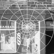
| A
log-polar grid with 16 rings and 16 wedges superimposed on a 180 x 180
pixel image. Each sample in a 16 x 16 log-polar image would be derived
from the grey levels in one segment of this grid. |
 |
|
The same image
sampled on a log-polar grid with 180 rings and 180 wedges, displayed on
orthogonal axes, ring number
horizontal and wedge number vertical, the origin at the bottom
left and top left corners (since the wedge number
wraps round). Moving up a column of
this image
corresponds to moving anticlockwise round a ring in the original
image,
starting at
3 o'clock.
Although log-polar samples are often displayed in this way, the
internal representation is no more "distorted" than any other image
representation - it is just a different mapping from array indices
to image position.
|
 |
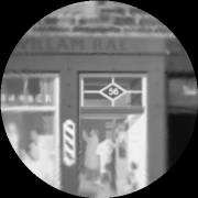
The
log-polar image above displayed with veridical
mapping onto the plane. (Bilinear interpolation was used to display the
image.) Note the loss on resolution near the periphery - e.g. the
number 54 on the door at the right - compared to the original
image. |
 |
In log-polar sampling, pixels are indexed by ring number R and wedge
number W, related to ordinary x, y image coordinates by the mapping
where (r, theta) are polar coordinates, (xc, yc) is the position of the
centre of the log-polar sampling pattern, nr and nw are the numbers of
rings and wedges respectively, and rmin and rmax are the radii of the
smallest and largest rings of samples. We also define rho = log r.
A log-polar sampled image is one whose samples are centred on points
mapping to integral R and W. In order to keep a pixel's nearest
neighbours in orthogonal directions at approximately equal
distances from it, the following constraint is needed
The log-polar straight line
Any straight line, not passing through (xc, yc), can be mapped into any
other straight line by a rotation (to make the lines parallel) followed
by a uniform expansion with (xc, yc) fixed. This property can be
exploited to allow easy detection of lines in log-polar images.
Essentially, the log-polar image of a straight line is taken as a
template and convolved with the log-polar image under analysis. Peaks in
the output correspond to the rotations and expansions that map the
template onto matching structures in the image, and so directly give the
parameters of detected lines [2].
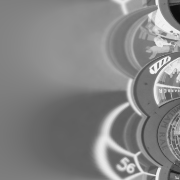
The equation of the straight line x=1 in log-polar coordinates is
and a graph of this equation is shown at the right (rho on the
horizonal axis, theta on the vertical).
If we convolve
the reflected log-polar image of this special straight line with the
image of a general line given by
then the peak of the convolution output will be
at  .
.
Since the template is the same size as the image, it is efficient to
perform the convolution by multiplication in the Fourier domain. It is
possible to find a closed-form expression for the Fourier Transform of
the straight line in log-polar space, and also to directly compute
the Fourier Transform of spatial derivatives of the mask.
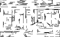
Example
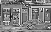
The
image at the right has been preprocessed to enhance local contrast
and remove very low spatial frequencies.
|
 |
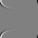
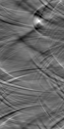
The image was then resampled
onto a log-polar grid with 128 rings and 256 wedges. This
resampled image was convolved with a straight line mask which
had been smoothed and differentiated with respect to R. The spatial form
of this is shown at the right, though the convolution was carried out
using the Fourier transform.
|
 |
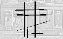
Local maxima
in the convolution output were found, and ranked by magnitude.
A line corresponding to each of these peaks is
plotted on the original image
at
the right. |
 |
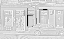
The lines found can be truncated to line segments by multiplying the
log-polar image
pixel by pixel with the spatial form of the convolution mask,
having first reflected and translated the mask to make it line up with
the detected line. The resulting array contains the values that would
have been summed to produce the convolution peak, if the convolution had
been carried out in the spatial domain. The size of these values
indicates how much each pixel of the image contributed to the peak. We
then simply project this array onto the W axis, by summing over all R
from 0 to nr-1 for each W, and threshold to find the line limits.
|
 |
An "eye
movement" strategy can be used to move the sampling centre
across the image to build up the representation of the image
structure. |
 |
Circle detection in the log-polar image
Since a circle through the sampling centre can be mapped onto any other
such circle by a rotation and an expansion, such circles can also be
detected by a convolution in log-polar space. Circles passing through
the origin are, of course, unlikely to occur by chance. However, if the
sampling centre is deliberately placed on a smooth boundary, possibly
using the output of log-polar straight line detection, then the circle
detected should approximate the osculating circle and the orientation
and curvature of the boundary can be estimated.
In fact
circles through (xc, yc) can be found for almost no additional
computational effort alongside straight lines.
Such circles are mirrored straight lines
in log-polar coordinates: the equation of the circle centred on
(xc+1/2, yc) is rho = log cos theta.
Thus the template shown above will match circles if it is
simply left-right reflected. A peak in the convolution output
gives the point on the circle diametrically opposite to the
sampling centre, and hence the circle's centre and radius.
Because of the symmetry between straight lines and circles, a single
Fourier transform pair can be used to detect both of them in a single
operation.
|
A log-polar image displayed on rho, theta axes, with the sampling centre
on the upper
edge of the car's rear wheel.
The car's shadow and the wheel show the reflection symmetry between
lines and circles.
|
 |
|
The result of convolving the image with a circle mask. Smoothing and
differentiation with respect to W were incorporated.
|
 |
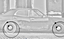
The circle corresponding to the maximum of the convolution output
(in white), along with
four other circles (black) generated the same way at different sampling
centres
(black dots), each chosen to be close to a curved boundary. Wheel arches
are found even though they are not exact or complete circles.
|
 |
References
[1] Weiman,
C.F.R. and Chaikin, G. (1979) Logarithmic spiral grids for image
processing and display.
Computer Graphics and Image Processing,
11,
197-226.
[2] Young, D. (2000)
Straight lines and circles in the log-polar image.
In M. Mirmehdi & B. Thomas (Eds.),
BMVC2000: Proceedings of the 11th British Machine Vision Conference,
11-14 September 2000, The University of Bristol (pp. 426-435). Also at
http://www.bmva.ac.uk/bmvc/2000/papers/p43.pdf


