This teach file complements FCS1 by relating the mathematical ideas described there to an important application: the analysis of a learning algorithm for feedforward neural networks.
This teach file is a complement to FCS1. It applies the mathematics in it to a single problem: the training of a multilayer feedforward nonlinear neural network (sometimes called a multilayer perceptron). Although this application is important in its own right, the purpose here is to give you some feeling for how ideas from calculus get applied to a real computational problem. In addition, you should get some idea of how the formal mathematical notation relates to the more concrete computational structures represented by neural networks.
You should not expect to be able to reproduce this whole argument. You should, however, be able to see in general terms what is going on. The idea of gradient descent is central to many computational systems, and the use of subscripts and summation to manipulate arrays of quantities in a concise way is well worth getting used to, since it translates readily into practical computer programs.
Two relevant books are:
Rumlhard, D.E. & McClelland, J.L. "Parallel Distribution Processing: Explorations in the Microstructure of Cognition", Vol. 1, MIT Press, 1986.
Hertz, J.A., Krogh, A. & Palmer, R.G. "Introduction to the Theory of Neural Computation", Addison Wesley, 1991.
Both of these carry out essentially the same development as this file, though more concisely.
Artificial neural networks (NNs) are formed by connecting individual units which very approximately correspond to neurons. Each unit receives some inputs from other units, or from outside the network, and produces an output which goes to other units or to outside the network. In an important class of NNs, the inputs and outputs are represented by real numbers, and each unit computes an output which is a function of its inputs. A common form for the function is described here; for justification see books on NNs, and remember that all sorts of other possibilities (such as networks with binary values only, or units with memory) exist.
In this section a single unit is considered. Suppose it has N inputs, which will be called x[1], x[2] etc. up to x[N]; the output of the unit will be called y, so we can write y = f(x[1], x[2], ..., x[N]) to express the fact that the output is a function of the inputs. The form of the response function f determines the behaviour of the network.
A very simple response function would be to just add up all the inputs. However, the unit may need to pay more attention to some inputs than to others, and this is achieved by first multiplying each input by a weight, which is a number expressing how strongly the input affects the unit. (I am regarding the weights as being associated with the unit they directly affect.) For each input x[i] there is a corresponding weight w[i]. The unit therefore combines its inputs by computing a weighted sum according to the formula
            N
    a  =  SIGMA  x  * w
          i = 1   i    i
where a is sometimes called the activation of the unit. The idea of a weighted sum is extremely common in many branches of science.
The unit could simply pass this activation to its output (i.e. it could set y = a). Such a unit is called a linear unit because if you plot y against any particular input x[i], keeping all the other inputs constant, you get a straight line.
If the weights are fixed, it is convenient to regard them as built-in to the response function f. However, the way that neural networks are trained is to adjust the weights to improve their performance. If we regard the weights as things that can be varied, it makes sense to regard the output as a function of the inputs and of the weights, or in symbols y = f(x[1], x[2], ..., x[N], w[1], w[2], ..., w[N]).
We will need to know later how a change in an input affects the output. For a linear unit (i.e. output = activation, or y = a), the relation is very simple:
c) y / c) x[i] = w[i]
(using the notation of FCS1). That is, the change in the output is just the change in the input multiplied by the corresponding weight. If the mathematics is not obvious, try writing out the formula for y explicitly for the case of two inputs (i.e. y = x[1]*w[1] + x[2]*w[2]). Then treating everying except y and x[1] as constants, use the ordinary rules for differentiation to find the derivative of y with respect to x[1]. Generalise the result to any input.
For working out learning algorithms, it is also useful to know how a change in a weight affects the output if the inputs are fixed. The mathematics is identical, and produces the result
c) y / c) w[i] = x[i]
i.e. for a particular input, the effect of changing a weight depends on how strong the corresponding input was.
It is the case that neural networks built from linear units have a very limited range of responses (e.g. they cannot produce an output that simply says whether two inputs are different from or the same as one another). However, one modification turns out to give the networks enormously greater computational power, and that is to make the relationship between the activation a and the output y nonlinear. Typically, instead of y = a, interesting neural networks use a relationship such as
             1
    y = -------------
        1  +  exp(-a)
This is sometimes called the logistic function. Note that a is just the weighted sum of the inputs, as for the linear unit.
It is not appropriate here to investigate why this is a useful choice, and anyway it is by no means the only possibility. We will take it as given, but we will have a quick look at its properties. The first thing to do is to look at its graph:
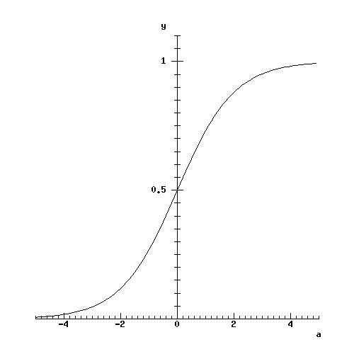
You can see that it is vaguely S-shaped. Functions with this shape are called sigmoidal functions (nothing to do with the sigma used to indicate summation). Note that the logistic function is merely an example of a sigmoidal function.
You can see that y is 1 if a is large and positive, and y is 0 if a is very negative. Thus if you ignore the bit in the middle this is a little like a binary function. However, y's changeover from 0 to 1 occurs gradually as a crosses 0 - one could describe this as a kind of softened or smoothed step function. (A step function would cause y to jump from 0 to 1 as a crossed some value called the threshold.)
Now we need to answer the same questions about how changing the inputs and weights affects the output of such a unit. This is done in two steps: first we ask how a change in an x or a w affects a, then we ask how a change in a affects y.
The first step has already been done. From the analysis for a linear unit, where a = y, we know that
c) a / c) x[i] = w[i]
and
c) a / c) w[i] = x[i]
The second step is to find dy/da. This requires the application of the rules of ordinary differentiation to the logistic function. I will not do this in detail here; if you want to see the steps involved, please ask. You have to know the rules for differentiating exp(x) and 1/x (x is just a general purpose variable here), and you have to apply the chain rule. The answer comes out as
    dy         exp(-a)
    --   =   ----------   2
    da       (1 + exp(-a))
(It is an ordinary derivative because a is the only thing that directly affects y - there's nothing that has to be held constant to do this calculation.)
You ought to be able to guess what the graph of this function looks like without using the formula, simply by looking at the graph of the logistic function and seeing what its slope does. The curve looks like:
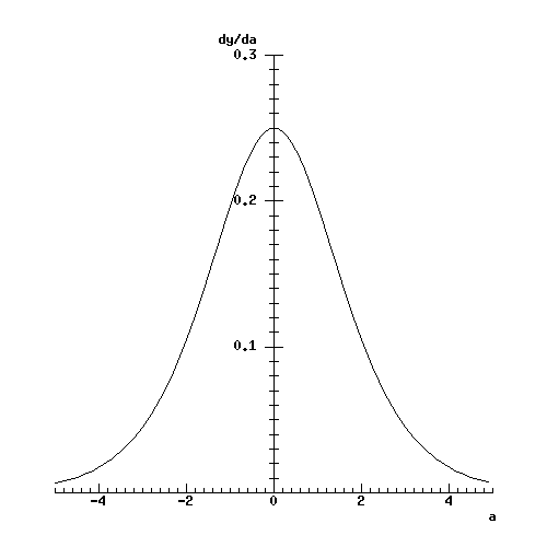
There is a computationally useful simplification of the derivative formula. It is possible to use the original formula for the logistic function to show that
dy/da = y * (1 - y)
If in some program, y has already been calculated, this gives a much faster way of finding the numerical value of the derivative than the formula that uses a.
Finally, the two steps are put together. You need to apply the chain rule, which says that
    c) y        d y     c) a
    ----    =   ---  *  ----
    c) x        d a     c) x
        i                   i
which gives
c) y / c) x[i] = y * (1-y) * w[i]
Similarly, one gets
c) y / c) w[i] = y * (1-y) * x[i]
This all looks fairly complex, but the final formulae are not too bad. They say how changes to the inputs or weights affect the output for this kind of nonlinear unit. They are in a form which allows them to be used in a program; such a program would have x, w and y available to it, so computing the partial derivatives would now be no problem.
These formulae imply that the unit's sensitivity to a change in a weight or an an input depends on all the other weights and inputs as well. If the unit's activation is close to zero (so its output is close to 0.5), it has its highest sensitivity. If the activation is strongly positive or negative, then the output is close to 0 or 1, y*(1-y) becomes very small, and so changes in inputs and weights have relatively little effect on the output. The unit is then said to be saturated. The possibility that some inputs can put a unit into saturation, and so prevent other inputs affecting the output of that unit, is an important aspect of the operation of neural networks with nonlinear units.
Neural networks are often trained using supervised learning. In this kind of learning, the network's output for a given input is compared with a target, which is somehow known to be the "right answer". The weights are then adjusted to make the output closer to the target. If the weights are adjusted after each new example of an input/target pair, the mechanism is called online learning; if the weights are only adjusted after a set of input/target pairs then batch learning is taking place. Here, online learning will be considered, as it is slightly simpler to understand.
To decide how close the network's output is to the target, on any particular presentation, an error function is used. For our single unit, the target will be called t, and the error is given by
                 2
    E  =  (y - t)
This function is chosen partly because E is always positive, and the bigger the difference between y and t, the bigger E is. It is clear that E is a function of y and t, and you will sometimes see this expressed as E = E(y, t). This is slightly loose usage, in that the same symbol, E, is being used for the name of the variable and the name of the function that computes it, but it is quite common and in practice does not cause confusion. You can read E = E(y, t) as "E depends on y and t".
Since E depends on y and t, and y depends in turn on the inputs and the weights, it is also true to say that E = E(x[1], ..., x[N], w[1], ..., w[N], t).
It is sometimes convenient to think of this error as an energy associated with the network. If this was a mechanical system in which y represented the position of a robot arm, say, and t represented a target to which it was supposed to move, then E would be a measure of the energy of a spring connecting the arm to the target. The spring would pull the arm to the target, reducing its energy in the process. This kind of physical analogy can be useful in analysing various kinds of computational system.
If we single two weights or inputs for special consideration, and keep all the rest at some fixed values, then it is possible to draw a picture showing E as a surface above a plane. Positions on the plane correspond to values of the two variables under consideration, and the height of the surface above the plane corresponds to the value of E. This is a useful conceptual tool, and it is often helpful to think of the error surface or energy landscape even when more than two things can vary; it is no longer possible to picture the surface then, as it exists in many dimensions, but the ideas from the 2-variable picture are still useful.
Now the standard question: how do changes in inputs and weights affect the error? What we need are c) E / c) x[i] and c) E / c) w[i], with the partial derivatives indicating that t is kept constant. Since we know how y depends on the inputs and weights, all that is needed in addition is to know how E depends on y. This is got by differentiating the expression above, which gives
c) E / c) y = 2 * (y - t)
(using the chain rule for simple differentiation). Then we can use (for inputs)
    c) E        c) E      c) y
    ----    =   ----   *  ----    =   2 * (y - t) * y * (1-y) * w
    c) x        c) y      c) x                                   i
        i                     i
Both of the things multiplied together on the right are already known, so the whole expression is easily found. The effect of weight adjustments can be calculated the same way to get
    c) E
    ----    =   2 * (y - t) * y * (1-y) * x
    c) w                                   i
        i
How can the single unit be trained? A standard and simple procedure is to select an input and a target, present the input to the unit, compare its output with the target, and then change the weights slightly to make the output closer to the target. This is repeated for a large number of input/target pairs. Because each individual change made is small, the total effect over a large number of trials is to make the unit's behaviour closer to the overall optimum (though the details are beyond the present scope). At the very start, the weights are given some random values.
One way of looking at this is to say that at some point in the training, we want to change the weights so as to take a step downhill on the error surface. This method is called gradient descent. Basically, each particular weight needs to be changed in the right direction to reduce E; the bigger the effect of that weight, the more it should be changed.
It might be helpful to think of this geometrically. Consider the error surface for a unit with only two weights, and some fixed inputs; this surface can be pictured as some kind of smooth canopy above a plane. The current weight values fix the position of a point on the plane and the point vertically above it on the error surface. Changing one of the weights means moving in one direction on the plane; changing the other weight means moving in a direction at right-angles to this. Such moves will take the point on the surface uphill or downhill, depending on how the surface slopes. The change in height for a small change in a weight is given mathematically by the partial derivative, and geometrically by the slope of a line on the surface vertically above the line of motion in the weight plane. It should be possible to convince yourself that if you make a change in each weight proportional to the slope in the corresponding direction, the total movement is directly uphill or downhill.
For a definite example, consider the case where the error does not depend at all on one of the weights (the corresponding input is 0). Then the error surface only slopes in the direction of the other weight, and it is clearly only appropriate to change the latter.
This can be summed up in the gradient descent learning rule, which is a core rule in neural networks, and the starting point for many other more sophisticated rules. It says (for online learning) that on each presentation, the adjustment to each weight should be proportional to minus the partial derivative of the error with respect to that weight. In symbols:
DELTA w[i] = - alpha * c) E / c) w[i]
This is just saying that we take a small step downhill in the error surface.
DELTA w[i] stands for the change in (adjustment to) w[i] that we are going to make. The minus sign means that we go downhill, not uphill, when we make the adjustment. The constant alpha (which ought to appear as a Greek letter) is used to keep the step small (in some sense) - in fact it used to be typically set to a value between 0.00001 and 0.2 by the experimenter and adjusted by trial and error, though there are now more principled and adaptive ways to determine a good value. The significance of the final part, the partial derivative or slope of the error surface, should be clear from the discussion above.
Now you are in a position to train a single unit. Putting everything together gives the adjustment to a weight after the presentation of an input as
DELTA w[i] = - alpha * 2 * (y - t) * y * (1-y) * x[i]
The output y would be calculated once using the basic formula for operation of the unit, then the adjustment for each weight would be calculated and applied in turn using the formula above.
One unit can only do so much. For really interesting behaviour, it's necessary to go to a network of interconnected units. Again there are many possibilities, and questions surrounding network topology are the subject of active research, but since the present purpose is to look at techniques for analysing networks, we will stick to one of the more amenable cases: the layered feedforward network.
In such a network, information flows from inputs to outputs, without any loops. The output of unit can never affect its inputs, which simplifies matters greatly. The units are arranged in layers, and each unit in any given layer gets its inputs from all the units in the previous layer (though of course it can ignore some of them by setting the corresponding weights to 0). (Sometimes the data from the rest of the world is thought of as coming through a layer of "input units", which simply pass their inputs on without changing them.)
First, take the case of a network that has a single layer (apart from any input layer). This will have one output for each unit in the layer. To analyse and train this network, the modifications to what we have done for a single unit are quite small, since essentially this is just like having a lot of units, all seeing the same inputs, but each doing its own thing.
The first change is in notation. We need to distinguish between the units, and to do this we have to use an extra subscript in some places. The output and activation of unit j will be called y[j] and a[j] respectively. There will have to be targets for all the units, so the target for unit j will be called t[j]. The weight for input i going to unit j will be called w[j, i]. The inputs are the same for all the units so they do not need an extra subscript.
The convention for the order of the weight subscripts might seem perverse (the destination comes before the source). However, it is convenient in the end, because it corresponds to the convention used for matrix notation. You will find this ordering used in the textbooks mentioned above, but other authors sometimes use the opposite convention - look out for which one is in operation.
You should draw yourself a diagram with the inputs, outputs and weights for a single-layer network marked.
It might seem that we need to have an error function for each output unit. However, it is much more elegant (and in the long run more general and useful) to have a single error function for the whole network. The nice thing about the error function for a single unit defined above is that the error function for the whole network can usefully be defined as the sum of the errors for the separate output units. That is, we write
                              2
    E  =  SIGMA  (y[j] - t[j])
            j
There is a slight shorthand for the summation here: when the range of j is not specified, it is assumed that j runs over all the appropriate units. This shorthand will be used quite often.
This is called the sum of squares error function. Sometimes a factor of 0.5 is put in front; this makes no real difference to anything, but reduces the number of factors of 2 that occur later.
Having defined E, everything now proceeds as for the single unit, except we have to keep track of which unit we are talking about. First we work out how a change in unit j's output affects E, by taking everything else as constant. By writing out the sum for the case of just 2 or three units, you should be able to persuade yourself that the result is just
    c) E / c) y   =  2 * (y  - t )
               j           j    j
That is, it is the same as for a single unit, except with a j subscript added as appropriate to indicate the unit. This is an extremely handy result - it simplifies the next stage, which is to find the derivative of E with respect to w[j, i]. But the analysis is now exactly the same as for a single unit, except for the extra subscripts. Thus a single layer is not really any more complex than a single unit, even though we have used a global error function which sums up (literally) the performance of the network as a whole.
Adding a further layer makes, as it happens, a big difference to the generality and power of this kind of neural network. It also makes it harder to work out how to adjust the weights; working out an algorithm for doing so was one of the major breakthroughs of neural network research.
The notation adopted here for the extra layer is non-standard, but makes it easier to follow what is going on. The new layer of units will go on the input side of the layer we have already considered. (I will refer to the original layer as the output layer.) Now x[i] will stand for the output of the i'th unit in the new layer and w[j, i] is the weight from the i'th unit in the new layer to the j'th unit in the output layer (so these symbols mean the same as before in connection with the output layer). The new inputs to the network as a whole will be called u[h] and the weights from the inputs to the first layer will be v[i, h]. Thus we have:
                                                                 targets
                                                                    |
                                                                    |
            weights                   weights                       V
 Inputs  ----------->  First layer -----------> Output layer ---> Error
                        outputs                   outputs
   u           v           x            w            y             E
This network is to be trained by gradient descent using the same rule as before. For a particular input, you can think of an error surface for E over a plane representing any of the weights in the system, the vs as well as the ws. We need to adjust all of them to go downhill on this error surface. The question is, what additional calculation do we need to do in order to carry this out?
Adjusting the weights w is exactly the same as before. The output layer doesn't care whether it's getting its inputs from the outside world or from a previous layer, so nothing changes for adjustments to w[j, i]. To adjust the weights v, however, we will need to know the slope of the error surface for these weights. This is the partial derivative written as c) E / c) v[i, h]. Finding an expression for this is the heart of the backpropagation algorithm.
A change in one of the weights v will affect the output of the first layer of units, x, which will in turn affect the ouput of the second layer, y which will in turn affect E. We therefore look at this causal chain to see if it helps us work out the influence of v on E.
First, we calculate how a change in one of the xs affects E. A change in x[i] will spread out to affect all the units in the output layer, which in turn all affect E. In terms of partial derivatives, this appears as
    c) E               c) E     c) y
    ----    =   SIGMA  ----  *  --- j                       (***)
    c) x          j    c) y     c) x
        i                  j        i
This is probably the most difficult equation in this file, and involves the most advanced mathematics - the chain rule for partial differentiation. Its value is that if you can see how the structure of this equation relates to the information flow in the neural network, then you are in a good position to analyse similar systems. The explanation of the chain rule in FCS1 might help here, as might textbooks that deal with partial differentiation. Writing out the expression in full (i.e. making the summation explicit) for a network with only 2 or 3 output units might be helpful.
Note the different roles of the i and j subscripts: j is a variable which is summed over, like a loop variable in a program, whilst i says which particular first-layer neuron's output we are talking about, and is more like an argument to a procedure.
Having written this down, we can evaluate it if we want to, since we already know the formulae for the bits of the right hand side - they both appear higher up this file. The first part is
    c) E / c) y   =  2 * (y  - t )
               j           j    j
(in section 4.1) and the second is
c) y[j] / c) x[i] = y[j] * (1-y[j]) * w[j, i]
which is modified from the equation in section 2.2 by putting in the j subscript to specify which output unit we are talking about. But in fact these details are not very important right now.
Because E depends on x[i] and x[i] depends on v[i, h], we have
    c) E        c) E      c) x
    ----    =   ----   *  --- i
    c) v        c) x      c) v
        ih          i         ih
There's no summation because v[i, h] directly affects the unit whose output is x[i] - no other variables get in the way.
We have just worked out how to get the first part of the right hand side. The second part is easy since it's just the same as working out c) y[j] / c) w[j, i] for an output unit, which we have already done. That is,
c) x[i] / c) v[i, h] = x[i] * (1-x[i]) * u[h]
So we have everything we need to evaluate the partial derivative of the error with respect to one of the vs, and hence to decide how to adjust that v.
That completes the mathematics for the backpropagation algorithm - we can now train a 2-layer neural net, by calculating the error gradients with respect to all the weights, the vs and the ws, and then applying the gradient descent rule to adjust every weight.
Why is this computation called backpropagation? The reason is the recursive nature of the central equation just above, marked ***. The derivative of the error with respect to the x outputs is found by using the derivative of the error with respect to the y outputs, together with a derivative which only depends on the y units. It is the quantity c) E / c) o, where o means the output of any unit (an x or a y), which is backpropagated across the layers. At each stage, the computation only involves one layer of units.
Suppose we put yet another layer of units into our network, again on the input side. Then we'd need the partial derivatives with respect to yet another layer of weights. To get these, we'd need c) E / c) u[h]. And to get that, we'd use
    c) E               c) E     c) x
    ----    =   SIGMA  ----  *  --- i
    c) u          i    c) x     c) u
        h                  i        h
This is just the equation marked ***, written for the next layer down. We'd have got c) E / c) x[i] when doing the previous layer, and c) x[i] / c) u[h] presents no problem now (we've done the same thing twice before). It's just the same computation again, and we could go on repeating it for as many layers as we like, working from the output to the input.
It was the realisation that this tractable computation was possible that allowed training of multilayer nonlinear networks to be carried out, and this in turn was one of the most important stimuli of their significant renaissance in the 1980's.
This rather long file has given an account of the mathematics behind training a multilayer nonlinear neural network. The essence of it is the equation marked *** - most of the rest is context for that: why it is needed and how it is used.
What this kind of mathematics is really about is keeping track of which variables depend on which others. If that is done, the partial derivative formulae should make some kind of sense, even if you could not carry out a detailed derivation of them. Relating the partial derivative formulae to the flow of information through the network is largely the point of the exercise.
Copyright University of Sussex 1997. All rights reserved.