Machine Learning - Lecture 7a Multilayer perceptrons
Chris Thornton
Introduction
A single weight vector can define a single, linear boundary.
This deals with data which show linearly separated classes.
But we often see more complex forms of patterning.
These seem to require a composition of linear
discrimantions.
For example...
Gain/loss comparison for loan-takers
Plot of all combinations of graduation/age (X axis) and
average career income (Y axis).
Val=1 implies net loss during replayment period.

More that one line needed?
One way of dealing with patterning of this sort is to use a
composition of linear boundaries to create a `frame'.
To achieve this effect, we can use techniques for
constructing and training multilevel neural networks.
Multilayer perceptrons (MLPs) are particularly of
use here.
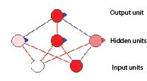
Multilayer perceptrons intro
In MLPs, we have a layer of weight vectors, each of
which represents a linear division.
Neural network terminology is applied, however.
The weight vectors are called hidden units; their inner
products are activations.
Applying error-correction to a hidden unit is described as
training the unit.
The value of each input variable is seen to be the
activation of an input unit.
Output units
There is then an additional weight vector at the top, whose
input units are the hidden units.
Datapoints for this output unit are the activations of
the hidden units.
Training the network
Given a suitably modified error-correction procedure, it is
then possible to train the whole network to produce a
desired composition of linear boundaries.
Indeed, for reasons explained below, we can train the
network to produce a composition with a curved boundary.
Implementation issues
To make MLPs work the way we want, we have to solve certain
problems, however.
One issue relates to activation.
Calculating activations as inner products produces a linear
effect, which limits the representational
power of the approach.
To get around this, we derive activation values as a
non-linear (sigmoidal) function of the inner product.
The sigmoid function
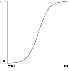 Also known as the `squashing' function for obvious reasons.
Calculating a sigmoidal activation
If  is the original inner-product, the activation is
then produced by
is the original inner-product, the activation is
then produced by

where  is the natural exponent (in Java = Math.exp(1))
Error backpropagation
We also need a way of applying error-correction in a network
of connected units.
This problem is solved by using backpropagation of
error.
The error of the output unit is derived as you'd expect, by
comparing the actual and target values in the usual way.
We then set the error of all hidden units in accordance with
the degree to which they contributed to the error of the
output unit.
This takes into account the size and sign of the
interconnecting weight, and the activtion of the input unit.
Setting hidden-unit error
One way to set the error a hidden unit is like this.

But it is actually more common to set the error using the
first-derivative of the activation.
This value is high for intermediate values of activation
(around 0.5) and low for extreme values (close to 1.0 and
0.0).
The effect is to allocate more error to units which are less
committed to a particular activation state.
The error formula for hidden unit i is then

Bias
Introduction of a sigmoidal activation function and the
allocation of error as noted makes it possible for
units to take on different roles, i.e. to `move' to
different parts of their weight space.
To get the full benefit of this, it is also common to
introduce unit bias.
Each unit is given an additional weight, which is imagined
to connect to an input unit which is always on (i.e., in the
1 state).
This weight gives units a bias towards high or low
activation, improving their ability to provide a distinct
contribution.
Momentum
Implementations of the MLP also often use some kind of
momentum arrangement.
Each time we update the weights for a particular unit, the
changes are a mix of any changes made previously, and the
changes currently dictated by the weight-update formula.
Weighting previous changes relatively more highly has the
effect of increasingly the stability of training.
MLP algorithm in full
- Configure the network of units and connections with
randomly assigned weights.
- Set the input-unit activations using the next datapoint.
- Set the activations of units in successive layers using
the sigmoid activation function.
- Calculate the error of the output unit.
- Apply weight-correction to units at this layer and
allocate appropriate error values to units in the layer
below (if there is one).
- Repeat step 5 for units at the layer below (if there is
one).
- If the datapoint is not the last in the dataset, repeat
from step 2.
- Exit if the average output-unit error is acceptably small.
Otherwise repeat from step 2.
Critical formulae
Basic activation (inner product) for unit 

Sigmoidal activation

Critical error formulae
Simple error for output unit  (given target activation
 )
)

Simple error for hidden unit

But we usually use first derivative of activation. So for output
unit

and for hidden unit

Full weight-update formula
The weight-update definition says how the change in the weight
in iteration  is related to the change in iteration
 .
.

where is the iteration,  is the learning rate and
 is the momentum term (normally 0.9).
This says that the change in the weight between unit and unit
is equal to
Demo - multi-layer weight correction
Demo using lossFromLoan data
Summary
- Neural network methods provide a way of finding and
representating complex forms of pattern.
- MLPs are a way of assembling a hierarchical structure of
units.
- Backpropagation of error is a way of training such
networks to produce a desired composition of linear
boundaries.
- Where a non-linear activation function is used, we have
the possibility of curved boundaries.
- Implementation is relatively complex.
Questions
- A combination of a threshold value and a weight vector
defines a line. What's the relationship between the
threshold value and the position of the line?
- When using weight-correction with a fixed threshold, how do we
choose the threshold value?
- When using an error value in weight-correction, should
the error value be calculated by subtracting the predicted
value from the correct value, or vice versa?
- Why is there a need to scale weight-changes in
weight-correction? (I.e, what's the point of the learning rate?)
- What is the effect of weight-correction on a linear
boundary in the case where the predicted value for the datum
in question is too high?
More questions
- How many weight vectors are there in a neural network?
- How does an input unit in a neural network work out its
activation level?
- Would the introduction of bias have any benefit in the case
where weight-correction is used with a single weight vector (i.e.,
unit)?
 ) plus the momentum value times the previous
weight change.
) plus the momentum value times the previous
weight change.