Machine Learning - Lecture 12 Perceptrons
Chris Thornton
Sample problem
     X       Y        CLASS
  (0-100)  (0.0-9)

    44      5.5    ->   H
    49      2.4    ->   M
    51      7.0    ->   H
    75      0.9    ->   M
    71      3.8    ->   H
    56      3.1    ->   M
    80      6.1    ->   H
    36      5.3    ->   M
Datapoint plot

Financial prediction example
 In this domain, data are financial quantities, e.g., daily
prices of commodities.
In this domain, data are financial quantities, e.g., daily
prices of commodities.
The aim is to predict future prices.
The goal is (usually) to maximize trading profits.
FTSE-100 movement classifications
 X is % increase in price of gold; Y is % increase in FTSE-100
Val=1: market rise sustained on the following day; Val=0:
rise not sustained
Linear separation of classes
Linear separation is the third of the simpler forms of
patterning.
Normally only seen with numeric data, i.e., continuous
variables.
From statistics, we have a simple and robust method for
modeling and predicting patterning of this form.
A little maths involved but the process can be visualised as
geometry.
Inner products
An easy way to define a linear boundary involves using
inner products.
Assuming datapoints are fully numeric, we
can calculate the inner product of any two by
multiplying together their corresponding values (and adding
up the results).
So if  and
and  are two datapoints, their inner
product is calculated as
are two datapoints, their inner
product is calculated as

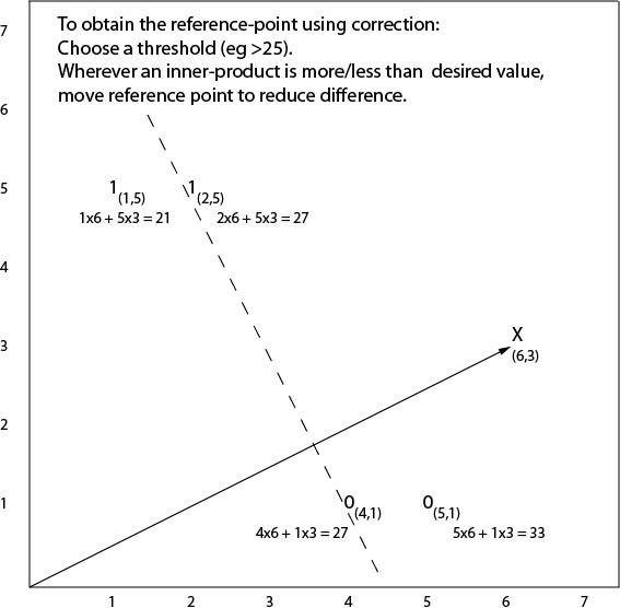
Boundaries from thresholds
If we look at how datapoints compare with some fixed
reference point, we find a nice relationship between inner
products and lines.
All datapoints for which the inner product with the fixed
reference point exceeds some given threshold turn out to be
one side of a line.
All other datapoints are on the other side.
This gives us an easy way of representing linear boundaries.
We can define them in terms of a fixed reference point and
an inner-product threshold.
Example
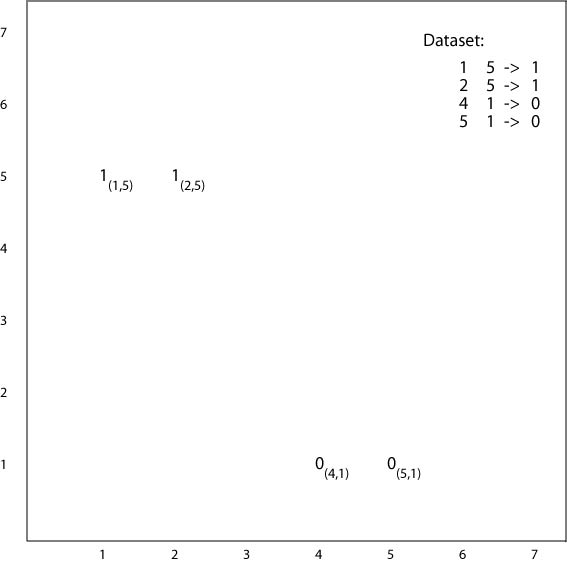
Reference point

Inner products
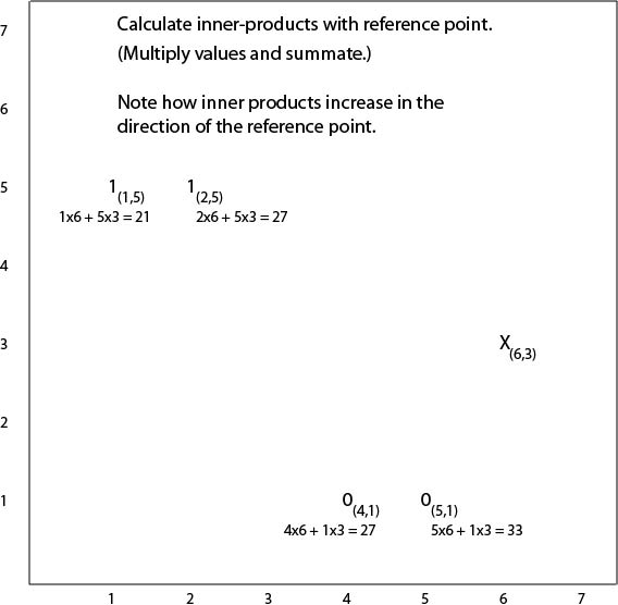
An inner-product threshold defines a line

Finding the boundary by error correction
The position of the linear boundary is a function of the
reference point.
Moving the reference point closer to the origin moves the
line in the same direction.
Also vice versa.
This suggests an incremental method for getting the line
into the right position.
- Get each datapoint in turn.
- If it's inner product is too high (i.e., it's outside the
line boundary), move the reference point back a bit.
- If it's too low, move the reference point out a bit.
- Stop if all datapoints are correctly classified.
Using error correction
Inner product too high

Inner product too low
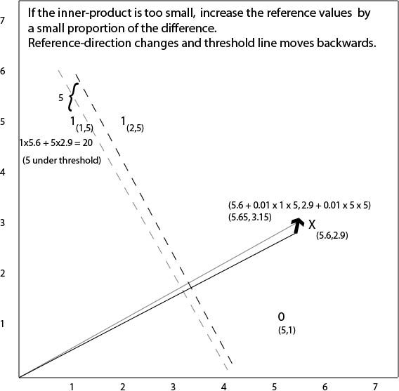
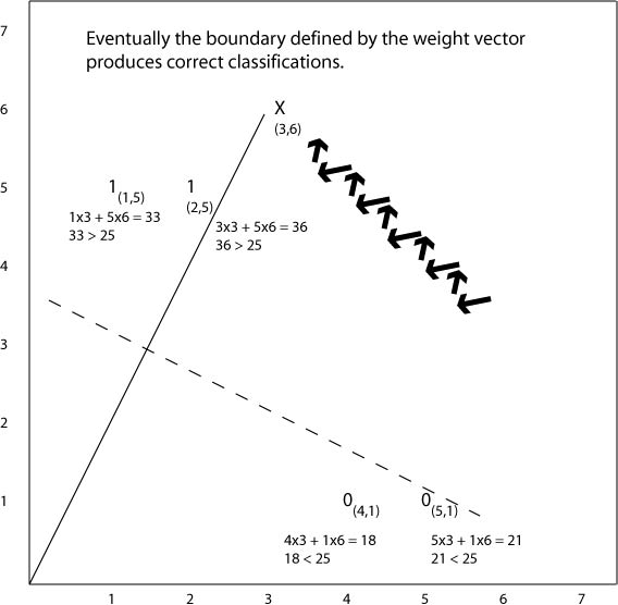
What happens in the end
Using an explicit error value
Instead of working in terms of overshooting and
undershooting, it is easier to use an error measure.
The coordinates of the reference point are termed
weights.
The reference point is called the weight vector.
The error for a datapoint is defined in terms of
a target value for that datapoint (e.g., 1 or 0).

Here  is the target value for the i'th
datapoint, and
is the target value for the i'th
datapoint, and  is the inner product for that
datapoint.
is the inner product for that
datapoint.
Using this definition we can get correction simply by
adding a proportion of the error.
This takes care of both over and undershoots.
Delta rule
Assuming the error  for datapoint
  defined
as above,
the new value for the i'th weight is
defined
as above,
the new value for the i'th weight is

where  is the i'th value from the datapoint and
 is the current value of the i'th weight.
Here, we also have a scaling parameter  , known as the
learning rate.
, known as the
learning rate.
This rule for finding a linear boundary is called the
delta rule.
Delta-rule error correction algorithm
- Set the weight vector to random values.
- Select the next datapoint and calculate its inner product with the
weight vector.
- Calculate the error.
- Derive new weights using the delta rule.
- Repeat from step 2 until average error is acceptably low.
Demo
Demo using stockMarket data
The neural network connection
Error-correction is interesting partly due to the connection
it makes between machine learning and neural networks.
Reference weights can be viewed as modeling the synaptic
weights of neural cells in brains.
The algorithm becomes a way of simulating learning in
neural networks.
In fact, this was one of the main ideas lying behind
innovation of the method.
Perceptron Convergence Theorem
In the 1950s, Frank Rosenblatt demonstrated that a version
of the error-correction algorithm is guaranteed to succeed
if a satisfactory set of weights exist.
If there is a set of weights that correctly classify the
(linearly seperable) training datapoints, then the learning
algorithm will find one such weight set in a finite number
of iterations
The main proof was developed in
Rosenblatt, F. (1958). Two theorems of statistical
separability in the perceptron. Mechanisation of Thought
Processes: Proceedings of a Symposium held at the National
Physical Laboratory, 1. London: HM Stationary Office.
Mark 1 Perceptron
Rosenblatt built a machine called the Mark 1 Perceptron,
which was essentially an assembly of weight-vector
representations for linear discriminations.
Noting the machine's ability to learn classification
behaviours (through error-correction), Rosenblatt went on to
make ambitious claims for the machine's `true originality'.

Minsky and Papert
Some while later, Rosenblatt's claims were strongly
questioned by Minsky and Papert, in their book
`Perceptrons'.
Machines based on linear-discriminant representations were
noted to be incapable of learning boolean functions such as
XOR.
  1 1 -> 0
  0 1 -> 1
  1 0 -> 1
  0 0 -> 0
This led to the so-called `winter of connectionism'.
Minsky, M. L. and Papert, S. A. (1988). Perceptrons:
An Introduction to Computational Geometry (expanded
edn). Cambridge, Mass: MIT Press.
Summary
- Linear separation is another simple form of
patterning.
- With numeric data, linear-discriminant lines are easily
defined using reference weight vectors and inner-product
thresholds.
- Incremental error-correction can be used to obtain a
separating line if one exists.
- Perceptrons are assemblies of linear-discriminant
representations in which learning is based on
error-correction.
Questions
- How can the concept of VC dimension be used to explain the
inability of perceptrons to learn the XOR function?
- Is it possible to achieve delta-rule error correction
through subtraction of error values? How would this be done?
- For some data based on two numeric variables, it turns out
there is a linear separation between the two
classifications. What can the slope of the line tell us
about the relationship between the two variables?
- What is left open in the the stopping condition of the
error-correction algorithm? How could we formulate a more
specific condition for a particular domain?
More questions
- A combination of a threshold value and a weight vector
defines a line in the data-space. What's the relationship between
the threshold value and the position of the line?
- When using weight-correction with a fixed threshold, how do we
choose the threshold value?
- When using an error value in weight-correction, should the
error value be calculated by subtracting the predicted value from
the correct value, or vice versa?
- Why is there a need to scale weight-changes in
weight-correction? (I.e, what's the point of the learning rate?)