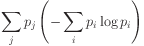
 values are the probabilities of
classes in the j'th subgroup, and
values are the probabilities of
classes in the j'th subgroup, and  is the
probability of a datapoint appearing in the j'th group.
is the
probability of a datapoint appearing in the j'th group.Decision-tree methods often use information theory for this.
The frequency with which an output appears can be seen as the probability of it being correct for all members of the group.
Frequency counts then become probability distributions.
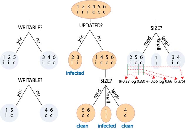
To find the best split, we take all the possible splits, and choose the one that gives the biggest reduction in uncertainty.
This is also the split that gives the biggest gain of information, i.e., the biggest improvement in the model.
Methods which work this way are said to use an information-gain heuristic.
How do we calculate an uncertainty for the split as a whole?
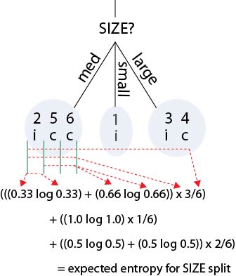
The solution is to calculate an expected uncertainty by weighting the uncertainty for each subgroup by its relative size (i.e., by the probability of it containing an arbitrary datapoint).
We then select the split that produces the biggest reduction in expected uncertainty.
Or equivalently, the biggest expected information gain.
Here, the values are the probabilities of
classes in the j'th subgroup, and is the
probability of a datapoint appearing in the j'th group.
Can it be used with numeric data?
In the standard algorithm, a split is constructed on a particular variable by creating one branch for each distinct value observed.
If we apply this to a numeric variable, we get one branch for each distinct number.
This may be fine with integer data.
The result may be a split with a huge number of branches, each of which creates a subset of just one datapoint!
The algorithm terminates immediately, having generated a lookup table in the form of a single branch.
Worst-case generalisation ensues, and there's a good chance the tree will not even classify an unseen example.
A simple idea is to find the observed value which when treated as a theshold gives the best split.
The resulting tree defines `large' generalisations in which each range of variable values is divided into two parts.
There is no risk of an unseen example being unclassified.
Imagine we have a variable representing age. The implicit structure may then be all to do with the four significant age groupings (0-20, 20-40, 40-60, 60+).
To deal with such situations, we really need the algorithm to put in a threshold wherever one is needed.
But how is this to be done?
Ideally, we should consider all possible ways of dividing the variable into subranges, and use the information heuristic to choose the best.
But the combinatorial costs are just too great.
This adds a number of features to the standard decision-tree algorithm.