Machine Learning - Lecture 8: Decision trees

Chris Thornton

Introduction to bias

Modeling involves finding and representing patterns in the data.

This means deciding what sort of pattern to look for, and how to represent it.

Learning methods always have a bias towards certain forms of pattern and representation.

A bias that is very specific is said to be strong.

Otherwise it is weak.

Because strongly biased methods are more focussed, they tend to be faster.

Weakly biased methods are more general.

The problem of bias-mismatch

A common problem in machine learning is bias mismatch.

This happens when the learning method is biased towards the wrong form of pattern, i.e., a form that does not feature in the data.

The result can be extremely bad performance in training or testing, or both.

Clustering methods

Clustering methods look for patterns which take the form of (hyper-)spherical groupings of similarly classified datapoints.

This is a common form of regularity.

But there are many contexts in which it is not seen.

Applying clustering methods in such cases is likely to be ineffective.

Demo

Demo involving ebaySales data with k-means clustering.

Ebay-Sales dataset

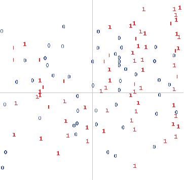
Rectangle structure

In the ebay data, we see data bunching-up in rectangular patterns.

This happens whenever specific values are significant in the classification of datapoints.

The effect is highly likely in categorical data.

It's also likely with numeric data whenever there are significant ranges or threshold values.

The wrong way to sort out bias mismatch

Applying centroid-based methods to data exibiting non-spherical forms of patterning, we have a bias mismatch that guarantees unsatisfactory results.

If we're not aware of what's going wrong, though, we may assume the answer is simply to increase the representational power of the method, i.e., increase the number of centroids.

The outcome can be then be confusing.

As we get closer to the situation of having one centroid per datapoint, performance on the training set improves.

But performance on testing data stays the same.

The `lookup table' effect

If we take this approach far enough, we end up with one centroid for each datapoint.

Performance on the training set is perfect.

But generalization is likely to be no better than would be achieved by random guessing.

We've fully replicated the data within the model.

The model then works as a kind of `lookup table' for the data.

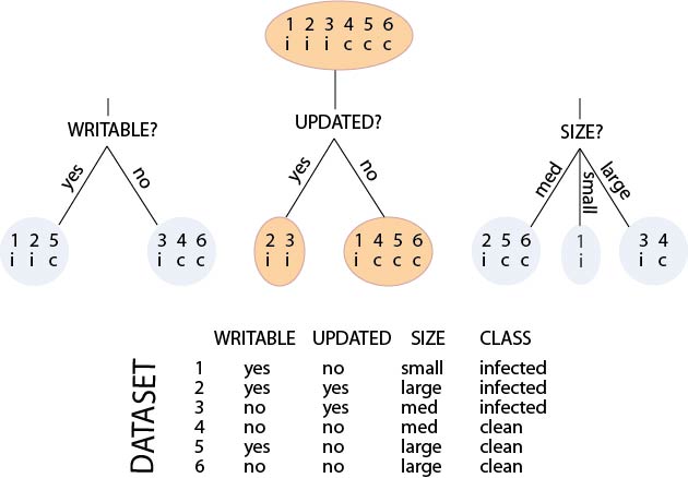
Decision-tree learning

Methods that are better suited for rectangular patterning are the decision-tree methods ID3, C4.5 and CART.

These incrementally construct a decision-tree, by repeatedly dividing up the data.

The aim at each stage is to associate specific targets (i.e., desired output values) with specific values of a particular variable.

The result is a decision-tree in which each path identifies a combination of values associated with a particular prediction.

The effect achieved is representation of rectangular patterns.

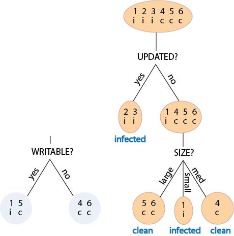
Worked example

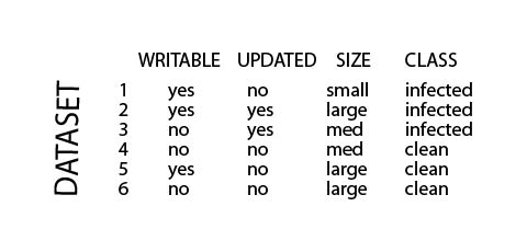
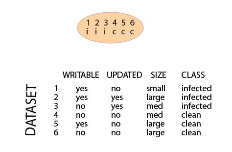
The data represent files on a computer system.

The task is to derive a model for virus identification.

Possible values of the CLASS variable are `infected', which implies the file has a virus infection, or `clean' which implies that it doesn't.

Initialisation of tree

Evaluating possible splits

Selecting the optimal split

Creation of a terminal node

Finalised decision tree

Derived rules and implied facts

Decision-tree algorithm

Define the initial node of the decision tree to be the set of all data. Label it `unfinished'.
Exit if there are no unfinished nodes.
Find the variable which best splits the data according to class value.
Divide the data up into subsets accordingly, creating a subnode for each one.
Label any subnode as finished if all its members have the same value of the target variable.
Repeat from step 2.

Golfing dataset

  type data\golf

  "Outlook    Temp  Humidity Windy    Decision
  sunny       75    70       true     Play
  sunny       80    90       true     NoPlay
  sunny       85    85       false    NoPlay
  sunny       72    95       false    NoPlay
  sunny       69    70       false    Play
  overcast    72    90       true     Play
  overcast    83    78       false    Play
  overcast    64    65       true     Play
  overcast    81    75       false    Play
  rain        71    80       true     NoPlay
  rain        65    70       true     NoPlay
  rain        75    80       false    Play
  rain        68    80       false    Play
  rain        70    96       false    Play

ID3 on the golfing data

  java Id3 golf
  Data: 10+4
  Variable names: [Outlook Temp Humidity Windy Decision]
  Most frequent output: Play

   Temp?
   |-- <=83.0
   |   |-- Play
   |-- >83.0
       |-- NoPlay

  Id3 #0 on golf R(10+4) 1.0 (100.0%)

Summary

Any ML method is biased towards particular forms of pattern and representation.
Poor performance is often due to a bias-mismatch.
Clustering methods are biased towards (hyper) spherical patterning.
Decision-tree methods are biased towards (hyper) rectangular patterning.
We tend to see this with discrete data, and whenever ranges or thresholds are significant in numeric data.
Addressing a bias-mismatch by increasing representational turns the model into a `lookup table'.

Questions

Would there be any way to modify a clustering method to make it more sensitive to rectangle patterning?
The decision-tree method requires the data to be expressed in the form of classified examples. To what degree does this limit its generality?
Will a tree produced by the decision-tree method always predict the correct classification for an example used for derivation of the tree?
Does it make any difference in decision-tree learning if we choose splits on the basis of expected information gain rather than on the basis of expected information?
Given two decision trees that both produce correct prdictions in all cases, how could we decide which one is better?