Machine Learning - Lecture 2: Nearest-neighbour methods

Chris Thornton

Brighton pier

Switchback

Data

Vertical axis is age; horizontal axis is alchohol consumption per week.
1s are riders who enjoyed the ride.

Machine learning using clumps

Let's say we'd like to use this dataset to learn a rule that lets us predict if someone will enjoy the ride.

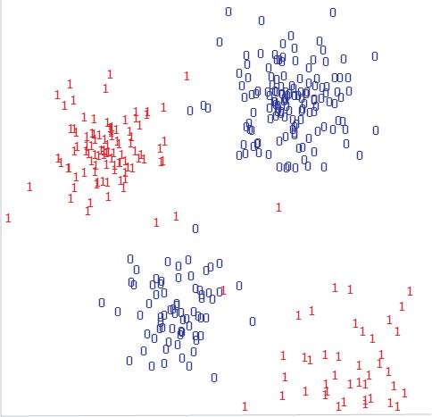
Enjoyment seems to be more likely if the individual's datapoint is near to a lot of 1s.

This suggests predicting enjoyment if the individual's datapoint is within one of the two clumps of 1s.

The data need to be modeled in a way that lets us work out which clump a particular individual falls near to.

Alternatively, we can take a shortcut and use the nearest neighbour method, also known by the acronym NN.

Nearest neighbours

To predict whether a particular individual will enjoy the ride, we work out the individual's datapoint and then find its nearest neighbour in the dataset.

If that nearest neighbour is a 1, predict enjoyment.
If it's a 0, predict non-enjoyment.

The nice thing about this is that we get around the need to do any work.

No looking for patterns.

No modeling.

k-nearest-neighbours

One problem with NN is that it can be derailed by `noise', e.g., a 1 right in the middle of a clumps of 0s.

To guard against this it is common to base predictions on several datapoints; i.e., we predict the value that is most common among k nearest datapoints.

This version of the method is known as k-NN, with k representing the number of nearest neighbours taken into account.

Implementing k-NN

To make k-NN work, we need a way of combining the values found in the k nearest neighbours.

With continuous data, the best approach is to average.

With categorical data, we can take the mode instead (i.e., most commonly seen value).

Measuring distance between data-points

We also need a way of measuring distance between datapoints.

The direct-line distance between two points can be worked out using the Pythagorean formula. It is the square root of the sum of the squares of the differences between corresponding values.

where is the i'th value of datapoint and is the i'th element of datapoint .

This is also known as the Euclidean distance.

Informally, it is the `as the crow flies' distance.

Euclidean distance example

Consider this dataset of two, 2d datapoints:

         VL      TC

  A      16      3
  B      17      4

Euclidean distance between A and B is then

City-block distance

The Euclidean measure treats the datapoints as if they were points in a physical space.

If this seems inappropriate, it is better to use the city-block distance.

This is just the sum of absolute differences between corresponding values.

Rather than measuring the `as the crow flies' distance, this measures the distance walking up and down blocks.

Nominal values

If we have categorial values (symbols or names) in the data, a non-numeric method of calculating distance is needed.

We can use use a hand-crafted differencing function.

More simply, we can just treat identical values as having a difference of zero and non-identical values as having a difference of 1.

Range differences

Note that these ways of measuring distances assume that all variables have the same range of values.

With real data, this is unlikely to be the case.

We need to standardize the ranges, through normalisation.

If we don't do this, distances between variables with larger ranges will be over-emphasised.

Normalisation

Normalization is a way of standardizing a set of numbers so each one is somewhere between 0.0 and 1.0.

We take each number in turn and subtract from it the minimum observed value.

We then divide by the observed range of values.

The result is a number between 0.0 and 1.0.

Normalisation example

Original data:

range of X is 10 (0-10) with minimum 0.
range of Y is 2 (-1.0-1.0) with minimum -1.0.

After normalisation

            X                         Y

  3 / 10 = 0.3      (-0.2 + 1) / 2 = 0.4
  4 / 10 = 0.4      (0.8  + 1) / 2 = 0.9
  9 / 10 = 0.9      (0.3  + 1) / 2 = 0.65

Turning symbolic data into numeric data

Nearest neighbour methods are usually implemented on the assumption of data being numeric.

But what happens if we get given some categorical data?

The easiest approach is just to convert them into numeric data.

Sparsification is a safe way of doing this.

It involves creating a new binary (0/1) variable to represent every non-numeric value of every original variable.

A new, continuous dataset is created by recoding the original data in terms of the binary variables.

Sparsification example

  COLOUR SHAPE

  red    ball
  blue   box
  red    box
  blue   post

Encode as 1s and 0s with values mapped to positions like this.

  red? blue? ball? box? post?

So red ball becomes <1 0 1 0 0>

Inductive inference

In machine learning, we formulate a prediction rule on the basis of patterns seen in certain observations.

Also known as inductive inference, this is the process on which scientific knowledge is assembled.

The basic approach of machine learning is essentially the basic approach of science.

This highlights the degree to which science is always a kind of guesswork.

Inductive inference is always uncertain

It's sensible to remember that predictions based on observed patterns are always inherently uncertain.

Scientific laws can turn out to be wrong, as we know from the example of black swans.

On the basis of observing many white swans in Europe the inductive inference was drawn that all swans are white.

Then it turned out there are black swans to be found in Australia.

Summary

Clumping is the tendency of data to bunch-up together.
This form of implicit structure can be exploited by learning rules which use the clumps as a reference.
The nearest-neighbour methods give the same effect for less work, i.e., no explicit model building.
But we have to be careful about measuring distances between datapoints.
Variables ranges may also need to be normalized.

Questions

The nearest-neighbour method avoids the need to build a model of the data. Does this mean it doesn't use a model of any sort?
When we sparsify some symbolic data, we usually end up with quite a few more variables that we started with. Is there any way of getting around this?
As a form of inductive inference, machine learning is like science---inherently unreliable. What steps do scientists take to ensure the reliability of inductive inferences?
What is the difference between Euclidean and city-block distance? How can we choose between them in a particular application?
What benefits might be obtained by normalizing the values of a discrete variable? How could the normalization be accomplished?