Chapter 1: Introduction
BugArt has roots in work done by Seymour
Papert, Daniel Bobrow, Wallace Feurzeig and others in the
1960s. These researchers developed a computer system called
`Logo', which though simple to use, gave access to the full
power of symbolic computation. (A history of logo is
available from the Logo Foundation website.)
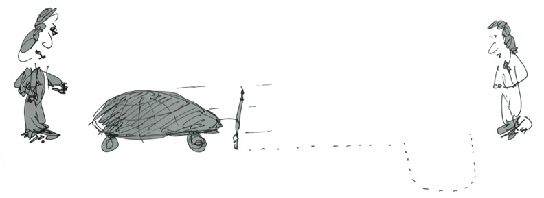
Logo was used to control a simple robot called the `turtle'. This was equipped with a downwards-pointing pen which scraped along the floor as the turtle moved about. Placed on a large sheet of paper, the turtle would then trace out a line showing its trajectory across the floor. On being given the command `FORWARD 50', the robot would move forward 50 steps. `RIGHT 90' would make it turn right ninety degrees, and so on.
Turtle motion evaluation scenario.
To get this programmable turtle to draw any sort of pattern it is necessary to give the right sequence of commands. Let's say the aim is to make the turtle draw a square. To get this, there would have to be a command to make the turtle move forwards a few steps and then turn 90 degrees to either the left or right. Then there would have to be a command to make the turtle repeat the sequence four times. The result would be a square drawn on the floor.
This idea of a computer-controlled turtle making marks on a surface is the inspiration behind BugArt. But whereas Logo treated robotic picture-drawing as a means to an end (learning about programming), for BugArt it is an end in itself. Logo was all about the programming. BugArt is all about the images.
The easiest way to get the hang off all this is to try
something out. As a first experiment, we'll work through
the process of creating a simulated robot (a `bug') and
getting it to generate an image of a square, just like in
the Logo example above.
First, click on the `Add com-bug' button from the main
window. Your pointer should now have a small, circular
object attached to it. This is a bug, or `com-bug' to be
precise. To place the bug into the arena, click down once
in the blank area of the main window. The bug will be
placed at the corresponding location.
You have now created your first bug and placed it in the
arena. From the BugArt point of view, the arena is the
`canvas' and the bug is the `paintbrush'. So you now have a
`robot paintbrush' sitting on your canvas waiting to do
something.
With com-bugs, there are two ways to control behaviour. You
can use a control panel of buttons or you can write simple
commands. For BugArt, it is best to use commands. Click once
on the bug to make sure it is selected, then press the
Open button from the right-hand panel. A dialog will
pop-up offering you a choice of using the button panel or
the program editor. It should look like this.
Initially, com-bugs always have the same program consisting
of the single command `move 50'. This ensures that an
unmodified com-bug will always try to move forwards fifty
units in each movement. To change this behaviour we need to
modify the program.
Click somewhere in the program editor and, after deleting
the `move' command already there, type in the following.
When run, this program will make the bug move 100 steps
forward before turning 90 degrees to the right.
To start the image-generation process, press the `Run'
button from the main window. This starts the simulation
running, i.e., it tells the system to activate any bugs in
the arena. The instructions you entered will then be
executed repeatedly and the bug will move continuously in a
rectangular pattern.
(Be careful to get the right `Run' button when you do this.
If you press the one in the program editor, rather than the
main window, the bug will execute the instructions once
only.)
With the simulation running, the bug should be moving in a
smooth, rectangular pattern. To produce an image, all you
need to do is press the `Show trails' button. The bug will
then leave a trail of color behind it and an image similar
to `First Box' will be built up.
By changing the program in the program editor, you can
change the way the image looks. For example, if you change
the turn command to
the shape will be eight-sided rather than four-sided, as in
`First Octagon'. Here the image build-up is shown in a nine
part sequence, known as a `cast-grid'. The cast-grid runs
left-to-right and top-to-bottom like English text.
The easiest way to change the body color of the bug is to
use the color sliders located in the bottom, right corner of
the main window. First select the bug and then move the
sliders to vary the intensity of red, green or blue in the
color. For example, for a more blue color, move the blue
slider to the right and the green and red sliders to the
left. If you try moving the color sliders with no bug
selected, it will be the color of the arena which is
affected. (This is how you can obtain a customised
`background' color.)
`Red Polygon' was generated using the com-bug we added
earlier, but with a turning angle of 40 degrees, a warm,
red, body color and a plum shade for the arena.
To see the difference these `noTrail...' colors make, try
setting the shell color to an ordinary value, e.g., `blue'.
When you re-run the simulation, the image will take on
a more tubular appearance, as in `Blue Shells'.
Note the fill effect at the corners. This results from the
fact that the square outline of the bug gets stamped out
repeatedly as the bug turns the corner.
Here, two `turn' commands are interleaved between two
`move' commands so as to achieve a swivelling `gun-turret'
action. This small increase in program complexity paves the
way for a very different image. Using a trail-making shell
color with a triangle pattern produces `Triangular Shells'.
This exhibits the `spirographic' quality so characteristic
of images generated using simple com-bug programs with
polygonal shells.
In the event of a collision, a bug is automatically turned
to the right, by an amount fixed by the setting of
`autoSwervingAmount'. (The normal value for this is 10,
meaning that a bug will be automatically turned 10 degrees
to the right any time it collides with the border of the
arena or another object.) This is quite a useful feature in
general because it stops bugs from getting stuck in corners
and `traffic jams'. But it also mean that objects which are
too large to move within the arena will tend to rotate
continuously.
The image `Arrow Confusion' exploits this effect in a simple
way. It was built up using a set of four bugs, all having a
user-defined arrow shape. The size of the bugs was increased
to the point where they were effectively unable to move at all
within the arena. The result was infinite rotation caused by
the continual application of auto-swerving.
As an illustration of the possibilities, `Acdc' uses three
kit-bugs using shapes roughly representing the letters `A',
`C' and `D'.
As a demonstration of shape editing, consider the derivation
of a chevron shape from a box shape, illustrated in the
figure below.
`Chevron Roller' was constructed using a chevron-shaped
com-bug and this command sequence:
`Exploding Hook' began with the introduction of a single,
kit-bug. The shape of the bug was changed to `box' and edited
so as to create an elongated, skittle shape. The body color
was set to `green'. Two copies of the bug were then created,
using the Copy and Paste buttons, and an image was cast from a
short simulation sequence. (The process of image casting is
described later on.)
To change its shape to `box':
To give the bug an invisible shell, the command would
be
In fact, `set' commands can be used to change any attribute
value you like. The commands
for example, would produce a long, thin bug with a
triangular shape. Commands like these can be interspersed
between `turn' and `move' commands so as to produce varying
patterns of variation.
If you're short of inspiration, try pressing the Randomise
button at the bottom of a com-bug window. This will generate a
random sequence of commands including a variety of `set'
commands. In many cases the simulation results will be
chaotic, with the bug tending to dart about the arena changing
its appearance in an erratic fashion. Sometimes, though, some
sort of visual coherence may emerge. For instance, the
following program yields the image `In Training', which shows
an interesting diagonal pattern.
Like all other chapters, this one concludes with a `pause
gallery'. The aim of this is to present a selection of
images constructed using the methods described in the
chapter. For this material, only a bare minimum of
explanation is provided. If you like, you can treat it as
an exercise to identify the methods that have been used to
build-up the underlying simulation.
This level of complexity can enhance the creative
experience. But it can also produce a sense of overload.
From the artistic point of view, there may be just too many
things that can be varied at any one time, while modulating
any single factor may have no noticeable effect on the final
product.
But there is a solution. BugArt is a machine-mediated process.
There is a computer in the loop. And we can make use of this
to lighten the creative load.
To see what the Modify window can do, try the following.
Use the `Add kit-bug' tool to add a kit-bug to the arena.
Increase its size using the Resize tool and set its shape to
`star'. Then make a copy of it (select and press Copy)
and add several instantiations to the arena (by pressing
Paste several times).
Running the simulation (with `Show trails' on) should now
produce some `shooting star' patterns, a little like `Star
Salute' perhaps. When first created, kit-bugs always try to
move towards whatever is nearest to them. The closer an object
is, the more they tend to move towards it. So, if one bug has
another bug as its nearest neighbour, both bugs will tend to
move towards each other.
To open the Modify window, press the Modify button from the
right hand panel. The window that pops-up should look like
this:
The value of the `shellWidth' attribute controls the width
of the object's shell. Changes in this can have the effect
of giving the image a less `jagged' appearance. `Pleasant
Thoughts', which uses a high shell width value, has a
distinctly fluffy appearance.
Of course it is easy to generate too much diversity this
way. Often an image will have more visual impact where bugs
retain clear commonalities. For example, images generated
using bugs of one shape often have a coherence that is lacking
in images combining different shapes.
As an illustration, consider `Dragon Tails' below, shown
first as a cast-grid and then as a single image. This was
obtained using kit-bugs, but with `color', `shellColor' and
`size' attributes randomised using through the Modify
window. Triangle shapes produce fan-effects when a
trail-making shellColor is used and the effect is more
striking when the shape is replicated across all the bugs
involved.
The value of a color attribute is normally a color name
like
`yellow' and `red'. But it can also be what is known as
an `RGB' (red-green-blue) value. This is just a sequence of
three numbers, each of which lies between 0 and 255.
The numbers specify the intensity of redness, greenness and
blueness in the color. An RGB value like
thus specifies a color made up from no red (first value), a
moderate amount of green (second value) and a maximum amount
of blue (last value). The notion of color combination should
not be taken too literally here. Although the RGB value
above might seem to specify a kind of greeny-blue color, it
actually denotes this:
on the other hand would denote perfect red because it has a
maximum red value and zero values for green and blue. In the
figure below, 21 examples are given showing randomly
selected colors with their corresponding RGB specifications.
You may have noted that RGB values are also produced when
you use the sliders to reset color. The resulting color is
specified in terms of whatever RGB values are currently
showing on the sliders.
With this setting, a value in a randomly-selected RGB spec
can be anything between 0 and 255, i.e., there is no limit
on what the color can be.
If you set the value of `randomColorRange' to
on the other hand, all the values will be taken from the
range 0-100 and the color will therefore be quite dark. The
figure below shows four examples of colors randomly selected
from this range.
random colors will be darkened shades of red because we have
specified the red value to be anything between 0 and 255 but
the green and blue value to be exactly 0. The result is that
the color will be made up of a certain intensity of redness
and nothing else. Some examples appear in the figure below.
i.e., a range which requires maximum values for red and blue
and anything between 0 and 255 for the green value. Examples
below:
will produce random colors which are shades of yellow, because
perfect yellow (in the RGB scheme) is an equal mixture of red
and green.
BugWorks will also let you use symbolic values in
these range specifiers. For example you can specify
as a way of constraining the green and blue intensities to be
identical to the red intensity (itself unrestricted). When
selecting a random RGB value using this specification, the
system will first choose a random number (from the range
0-255) for the redness and then---because an `R' appears in
the G and B positions---will use the same value for green and
blue. The result will be that random colors have identical R,
G and B values. They will therefore be shades of grey (i.e.,
darkened shades of white). Examples below:
will ensure that random colors have a green value which
is randomly chosen from the range 100-200, a red value
which is identical to the green value and a blue value
which is the result of subtracting 50 from the green
value.
will ensure that random colors have a blue value chosen
from the range 80-100, a green value chosen from the
range 0-50 and a red value which is twice the blue
value. The end result is a muddy red color, as in the
examples shown below.
This will ensure that random colors have a red value in the
range 200-255, a green value which is half the red value
and a blue value of 90.
Symbolic expressions using multiplication and division make
it possible to preserve proportionality between red, green
and blue intensities. And it is this, more than absolute
intensity, which is key in color perception. Two quite
different colors will often be perceived as being the `same
color' provided the red/green/blue proportions are the same.
(If you want to explore the effects of changing these range
specifiers, there is a useful shortcut. In the Settings
dialog, simply enter the word `random' as the value of any
color range and the system will then
invent a range
specifier on the fly. Of course, you then have two levels of
randomness to conjure with. First there is the random choice
of range specifier. Then there will be selections of colors
chosen randomly within the specified range. If this is
making your head hurt, move on quickly.)
But the Modify window is far from being the only way in
which BugWorks supports randomisation. As we have seen,
there is also the Randomise button which appears in each
com-bug program editor. This can be used to generate a
random program of `move', `turn' and `set' commands. The
image `In Training' was generated in this way.
As noted, com-bugs given randomly-generated programs of this
sort tend to behave in a wild fashion, darting around in all
directions, repeatedly changing shape, color and size. The
visual effect can be extremely `busy'. `Beserker' is a not too
offensive example.
On the whole, though, this approach does tend to generate
too much disorder. To achieve the best visual effects it is
often necessary to find some way to emphasise symmetries
and commonalities. One of the easiest ways to do this is to
have a set of com-bugs all use the same program. The
easiest way to to achieve this is simply to copy and paste
the relevant program from one program editor into another.
`Depression With Holes' was generated this way. It uses
four com-bugs following the same program of commands. The
behaviour generated by all four bugs is identical, except
with respect to its location within the arena.
This will cause the bug to move forwards some number of
steps randomly chosen from the range 0-7. (You can of course
use any number you like instead of 7.) You can also use
these random values in turn commands and set commands. For
instance,
will cause the bug to turn to the right by some number
of degrees randomly chosen from the range 0-90.
Colors can also be specified using random values in
set commands. The most obvious way to do this is to create
three random intensity values, making up an RGB value.
Intensity values are numbers between 0 and 255, so color
randomisation would be achieved by
This will set the bug's color to an RGB value randomly
selected from all possible RGB values. To create colors of
particular shades, simply modify the randomisation ranges.
The command
is likely to produce a fairly dark shade of red, because the
red value will be chosen form the range 0-255 while the
green and blue values will be chosen from the more
restricted range 0-80.
The letter `R', 'B' or `G' can be attached to the end of any
color attribute so as to access the red, blue or green
intensity of the color independently. To randomise the blue
intensity of the bug's shell color, the command would be
To set the red intensity of the bug's color to a randomly
chosen value from the upper part of the range, the command
would be something like
Sometimes, what we want is to set the bug to use a color
generated according to the current setting of
`randomColorRange'. As noted in the previous chapter, this
setting (accessed via the main Settings dialog) controls
the range in which random colors are generated. To obtain a
color selected from the range defined by this setting, use
the the `randomColor' variable. For example:
Working in much the same way as the `randomColor' variable,
there is also `randomShellWidth'. The value of this is a
number randomly generated within the range defined by
`randomShellWidthRange' (normally 1-5). So a command such
as
will set the bug's shell width randomly but within the
range currently defined by `randomShellWidthRange'. (Tip:
to eliminate shells from all bugs in your simulation, set
`randomShellWidthRange' to `0-0' and then randomise the
shell widths of all the bugs.)
With no random values used, com-bugs are likely to
fall into some kind of cycle, in which they carve out a
regular pattern around a central point. Given enough time,
the effect will then be to fill-in a roughly spherical
region of texture. This will often produce floral patterns.
`Petallic' is an example.
generates the image `Random Twisting'. (A custom `coffin'
shape is used here.)
For BugArt purposes, the Reproduce button offers little more
than can be achieved using the Randomise button in the
Modify window. So no great effort should be made to come to
terms with its use. As ever, the quality of results obtained
through use of this device depends very much on the quality
of the ingredients which are fed in. `Hand of Hooks' is a
reasonably appealing product.
But the way randomisation is used in BugArt is quite
different to the way it is used in the British Museum
Algorithm. In BugArt, randomisation does not impact the
final output (the image) directly. Rather, it impacts the
functionality of the mark-making agents. Randomisation is
certainly used to inject novelty, but this novelty is then
moulded and refined by other processes. Randomisation in
BugArt, then, is much more like what happens in Jackson
Pollack's `drip and splash' method, say, than in the
British Museum algorithm.
The pause gallery for the chapter now presents a range of
images whose construction involved randomisation of some kind.
The roller images `Paint it Mauve' and `Paint it Yellow'
demonstrate the way settings of `randomColorRange' can be used
to modulate color randomisation. `Walker' showcases the use of
behaviour duplication in a set of com-bugs. `Headache'
features an interaction between a kit-bug and a randomised
com-bug, while `Keep off the Beanstalk' and `Cool Deviance'
explore use of custom shapes and shell width variation.
With this setting, random colors tend to have large
blue values, smaller green values and negligable red
values, tending to produce a mauve or purple shade.
Changing the random ranges and re-randomising the bug
colors gives a different look. `Paint it Yellow' was
produced using the same simulation but with colors
randomised in the range `150-255 R-20 R/4'.
`Purposeless Furry Balls' is another example. Cast from a
com-bug simulation fearturing
several random turns and moves, this
exhibits a single random walk, kept within the confines of
the arena by auto-swerving.
This is a nice and simple way to generate images. But it's
not the best way. A more powerful method involves saving a
simulation as a movie, and then `casting' an image from the
movie. Doing it this way gives you more control over what
appears in the image. It also lets you save the image in an
electronic form for inclusion in web pages. (Nearly all the
images in this book were created as movie casts.)
In order to cast an image from a movie, we first have to
record a simulation sequence as a movie. This involves using
the BugWorks record facility (only available in the full
version of the system). The procedure is exactly as used on a
tape recorder. To record a simulation, simply press the Record
button. The simulation will then be activated, just as if you
had pressed Run, and everything that happens will be recorded
until you press Stop.
At this point, the BugWorks movie-player window will pop-up
along with the Save-movie dialog. For convenience, place the
dialog somewhere below the movie-player window, as in this
screenshot.
To establish a good `showFrame' for the movie, first reset
the movie to its starting state, by pressing Reset or by
double-clicking the window. Then, while holding the CTRL
key down, drag the pointer horizontally across the window
from left to right. This will have the effect of slowly
advancing the movie, i.e., of `scrubbing' it forwards.
Dragging in the other direction has the opposite effect: it
will retard the movie, i.e., scrub it backwards.
During these operations, the current frame number is
displayed in the top, left corner. It is this number which
shows you what the `showFrame' value should be. Once the
movie has been advanced to a satisfactory point, i.e., once
the image has a satisfactory appearance, simply copy the
number showing in the top, left corner into the `showFrame'
field of the Save-movie dialog. To check the new value has
been registered, press Show. The movie-player will
redisplay the movie up the selected frame. If the final
image is what you expect, you can press Save to save the
movie.
For example, consider the `Cracking Up' image. This was
cast from a movie of a simulation involving two, triangular
kit-bugs.
On further examination, the image at this point seemed a
little `undeveloped'. So it was further advanced to frame
60. At this point the window looked like this.
The value 60 was then entered as the `showFrame' value and
the movie was saved to disk using the Save button.
Once these settings have been fixed, the Save button is
pressed. A file dialog pops up allowing you to specify a
name for the movie. The movie is then saved to disk, from
where it can be re-played (and if desired, re-cast) at any
time using the Movies button in the main BugWorks window.
When displayed in a web page, the movie will always be
advanced to the relevant `showFrame', thus re-creating the
desired static image.
Changing the zoom setting is a good way to crop off
unwanted white-space around the edge of the arena. It can
also be used to focus down on a particular detail of the
simulation. Zoom and scrollbar settings are saved along
with the movie and are re-created whenever the the movie is
played or displayed as an image.
The movie-player allows cast-grids in the standard 3x3
format to be generated automatically. Clicking in the
window with the ALT key held down will automatically cycle
the movie-player through its display modes, one of which is
the cast-grid mode. (The other mode simply runs the movie
with trails switched off.) While in cast-grid mode, the
player will display the movie as a 3x3 grid of casts, each
one showing a slightly longer initial sequence from the
movie.
BugArt turns this convention around, drawing the process of
framing right into the heart of the creative process
itself. Provided with an extra spatial dimension (courtesy
of the movie-player's zoom mechanism) and an extra temporal
dimension (courtesy of the frame-marker mechanism) the
process is transformed into a new tool of image
enhancement.
There is absolutely nothing to stop the casting process from
having a direct influence over the simulation design and
operation. In fact, this is really what is expected. For the
bugartiste, is is not so much a case of the tail wagging the
dog; it is more a matter of liberating the potential synergy
between two mutually reinforcing processes.
The images included in this chapter's pause gallery provide
some illustrations of the way the relationship between
casting and simulation-making can be negotiated. In each
case, the image is first shown as a cast-grid and then as a
single image, with the cast-grid representation using a
neutral cast, i.e., no zoom and `showFrame' set to zero.
The aim is to highlight the impact casting has on the
underlying simulation product.
In some cases, cast-grids may have a visual appeal which
exceeds that of the original image itself. Of the two
versions of `Two Towers' shown below, it may be felt that
it is the cast-grid which has the greater visual impact.
Use the `Add kit-bug' tool to add a kit-bug to the arena.
Making sure the bug is selected, press Open. The window
which pops up will show a top-down, plan view of the bug's
components, as below.
Note how the left-hand sensor is joined by a line to the
right-hand wheel, while the right-hand sensor makes a
connection to the left-hand wheel. These lines represent
connections which carry signal from one component to another.
The bug is said to be `cross-wired' because signal coming from
the sensor on one side goes into the wheel on the other side.
The way the simulation works, the amount of incoming
signal to a wheel controls the wheel's speed of
rotation. Since the amount of signal generated by a
sensor depends on the closeness of the nearest object,
we have a tight linkage between the relative position
of other objects in the arena and the speed with which
the two wheels rotate.
If the closest object is on the left hand side of the bug,
the left-hand sensor will generate the most signal. This
will cause the right-hand wheel to turn fastest. The
right-hand side of the bug then travels faster than the
left-hand side and the bug turns to the left. This is the
side where the closest object is. If the closest object is
on the right-hand side, the effect is reversed. Now it is
the right-hand sensor which generates the most signal and
the left-hand wheel that turns fastest. The bug turns
towards the right which is, again, the side where the
closest object is. The behaviour is beautifully simple and
robust. But it is really just a big knee-jerk reaction---a
simple consequence of the fact that each sensor is
connected to the wheel on the opposite side of the bug.
The main appeal of the standard `cross-wired' bug from the
BugArt point of view is that it generates a smooth, curving
trail for very little effort. It is possible to generate
smooth curves using com-bugs, of course, but the process is
more cumbersome and curvature tends to remain static. The
arc carved out by a cross-wired bug, on the other hand, will
show a curvature which varies automatically as it turns
towards whatever it is being attracted to. The curvature is
greatest when the bug is side-on to the attracting object.
As the turn is completed, the curvature decreases, an effect
illustrated in `Simple Approach'.
The standard, cross-wired kit-bug will try to move towards
the closest object, regardless of what that object is. This
means that it will happily move towards another bug. Two or
more cross-wired bugs placed into the arena will therefore
tend to chase each other around. As we have seen, these
chases can create swirling vortices which quickly become
complex. Very often these chases will degenerate into
simple race-track patterns. `Basic Chase' is an
illustration of the effect.
To experiment, open a kit-bug and press `Show tools' to
bring up the tool bar. In addition to the usual Grab tool,
you will see a Connect and a Resize tool. The Resize tool
works the same way it does in the main window. It is useful
for resizing wheels and this is certainly the easiest way
to fine-tune the speed of a bug. (Bigger wheels produce
more speed.) The Connect tool is used for creating and
deleting connections between parts. (Drag between parts to
make a connection. Drag again to delete it.)
In addition there is an `Add' tool for every type of
component that the system implements. These include
batteries, sensors, wheels, junctions, transformers,
processors and neurons. By adding parts to a bug and
creating connections between parts, it is possible to obtain
a large variety of behaviours.
For example, take a kit-bug and try deleting both sensor-wheel
connections. Then add a battery and connect it to just one of
the wheels. When you run the simulation, the bug will rotate
on the spot because the internal arrangement ensures that only
one wheel receives any signal.
Now introduce another battery with a connection to the other
wheel. Use the Properties dialog to reset the battery's
activation value to 0.5. When you run the simulation the bug
should now carve out some sort of arc. Although both wheels
are receiving signal, one signal is higher than the other.
From the BugArt point of view, manipulation of behaviour
through innards-editing is not an immediate concern. If you
want to investigate use of parts in more detail, access the
BugWorks tutorial (via the Tutor button). This goes into full
detail on all features of the system. For current purposes,
basic operations using batteries, sensors and wheels will be
sufficient.
With standard kit-bugs, there will be trails made by the
wheels and the sensors. But there will also be trails made by
the connecting channels. These are normally drawn in shades of
red, with the intensity of red indicating the amount of signal
passing through the channel. (Negative signal is represented
using shades of blue.)
`Wormingoes' is an attempt to illustrate what can be
achieved purely on the basis of channel coloration. It uses
two kit-bugs with the standard configuration of cross-wired
wheels and sensors. The sensors have been pulled well out
from the body so that they protrude a considerable distance.
The wheels have then been moved closer together to achieve
more vigorous turning. Finally, all wheels and sensors have
been made invisible so as to allow the color effects to
dominate.
This specifies the range of RGB values to be used for
representing signal levels. The spec uses the same
left-to-right conventions as an RGB value. The first item
(255) represents the range of red intensities. The second
item (0-255) represents the range of green intensities and
the third item (0-255) represents the range of blue
intensities. This particular setting ensures that channel
colors will range from
which is perfect red, to
which is perfect white. Signal levels will be represented,
then, using shades of color between red and white.
To obtain different channel coloring, simply change the
setting of `activationColorRange'. In `peepingBlueAndGreen'
for example, the setup from `Peeping Pink' was re-used but
with the value of `activationColorRange' set to `0 0-255
0-255' to ensure that activations were displayed using
shades of green.
Images constructed using unmodified kit-bugs with parts
showing are often complicated, zip-like patterns. `Zipper
Knot' and the other `Zipper' images below are typical casts
from this sort of setup.
Where com-bugs are used, the attribute `moveStep' directly
controls the size of the step that the bug makes in each
cycle, while `turnStep' controls the angle of turn that can
be completed. By setting a com-bug's `moveStep' to a high
value, we effectively force the bug to jump around the
arena. As a simple example, `Niner' was constructed from a
triangular com-bug using the program `move 100' with a
`moveStep' of 2. Note that the `moveStep' value is
interpreted proportionately with the size of the bug. The
default value of 0.2 implies that com-bugs move in steps
which are 20% of their body length. The value of 2 thus
causes the bug to make jumps which are twice its length.
In an ideal BugArt system we would have complete control
over all `physical' properties of the underlying surface.
Unfortunately, although BugWorks allows control of color it
provides no way of controlling more subtle qualities such as
texture and viscosity. However, surface-related effects can
sometimes be achieved through the introduction of passive
objects.
BugWorks provides buttons for adding `mud', `rock' and
`debris'. These objects are like bugs except that they
don't do anything, which is what makes them `passive'.
However, each type of object permits a different type of
interaction:
Mud objects are added using the `Add mud' tool. Once added
to the arena, mud can be resized and reshaped to suit, just
like any other object. More interestingly, mud can be given
a customised `solidity' value, i.e., it can be made more or
less solid. Using the Properties dialog, the solidity of the
mud may be set to any value between 0 (implying no solidity
at all), 0.5 (reasonably penetrable) to 1 (totally
impenetrable). An intermediate solidity value is best since
it nurtures more complex interactions.
The speed of a bug moving through a patch of mud is reduced
depending on the mud's solidity value. But the most
interesting effects occur when a bug just `nicks' the edge of
a patch of mud. The side which falls into the mud is slowed
down more than the side which is still outside it; the bug
slews towards the centre of the object. If the mud object is
circular this can create wave-like effects.
Demonstrating the effect in a simple way is `The Saddle'. Here
a standard, bug with a chevron shape produces an unusually
complicated motion through the arena. The behaviour of the bug
is being influenced by the presence of three large blobs of
mud, all of which have been made invisible. As it crosses out
of an area occupied by some mud, one of the bug's wheels is
suddenly able to move more rapidly. The bug executes a U-turn,
turning back towards the mud's center.
`Arrow Eye' is a case in point. Here two arrow-shaped
kit-bugs are caused to circle a single rock
object. For purposes of creating this image it was
essential to modify the bugs so that they would be
attracted only to the central rock and not to each
other.
The general principle is that we add something to the
`inputSources' attribute which says what properties
something has to have in order for it to register as a
stimulus. The annotation to the sensor spec must specify the
name of an attribute followed by its required value, all
enclosed in square brackets. The annotation effectively adds
a constraint to the specification. Sensitivity is then
narrowed down to whatever objects meet the constraint.
To add a filter to a sensor, first open a Properties
dialog on the sensor. Select the part and then press
Properties (or right-click the part). The value of the
`inputSources' attribute will show up as
If you want the sensor to be sensitive only to rock,
you would need to change this to
If you wanted the sensor to be sensitive only to
yellow objects, you should use
and so forth.
Use of more than one constraint is allowed. For
example, a constraint which limits sensitivity to
objects which are both triangular and blue would be
To focus sensitivity onto a single object, specify the
appropriate name value as a constraint. For example, to
achieve a sensor that is only sensitive to the rock called
`rock3' you would use
`Selective Chase'
was cast from a simulation involving three
standard kit-bugs with filters used in all six sensors. The
three bugs were given two pairs of sensors each, with one
pair cross-connected to the wheels and the other uncrossed.
Filters were then added to each pair to cause them to
respond only to bugs of a particular color (either red or
yellow). In other words, the bugs were configured to
approach bugs of one color but flee from bugs of the other.
`Upstairs Downstairs' illustrates the use of sensor filters
to modulate responses to passive objects. The simulation has
been set up here to contain a number of rock objects
arranged in a staircase pattern. The body color of all the
rocks is
`invisible'. But the two rocks at either end of the
staircase have a green `shellColor'. The bug has the
standard, cross-wired configuration, a box shape and a
red-brown color. Its sensors, however, have been modified so
as to be sensitive only to objects with a green
`shellColor'. In other words, the `inputSources' value, in
both cases, has been specified as
The result is that the bug is drawn towards the blocks at the
ends of the staircase. But inevitably it collides with the
intermediate blocks along the way and is `auto-swerved' away.
The result is a `bouncing down the stairs' effect rendered
upside-down.
Anyone familiar with the system will have noticed that it
can be used as a kind of paint box. With trails switched on,
dragging objects across the arena leaves a streak of color.
So, it is possible to draw a picture by hand simply by
dragging a suitably configured object around the arena. To
illustrate,
`Bugart' is my attempt to write the book's title
using a small piece of brown rock.
There is the potential, then, for a cooperative style of
work, or what I call the `hands-on-top' approach (because
it's somewhere between `hands-on' and `hands-off'). In
following this approach, we can bring into play all the
techniques explored so far. But we can also attempt to
modulate the image-generation process using the facilities
provided by the BugWorks user interface.
To try your hand at this, proceed as follows. Use the
relevant tools to add a small rock and three or four
kit-bugs to the arena. Start the simulation running, grab
the rock and move it around a little. When they're not
chasing after each other, the bugs should now attempt to
chase the rock you are moving around.
Remember that kit-bugs move towards the closest object. So
moving your target object in front of a bug should capture
its `attention'. Once all bugs have been captured in this
way, the effect will be something like a swarm of bees
buzzing around an open jam jar. `Spagarti' is the result of
my attempt to write `bugart' again, while being pursued by
four `captivated' kit-bugs.
Casts taken from a follow-me scenario may be more striking
if the target object is left out of the image altogether.
You can achieve this effect by giving the target an
invisible shell and body color. However, in this case you'll
need to remember where you put it so that you can re-grab it
at the start of the image making process! If you lose it,
use the `Select all' button. This will put boundary
highlights around all the objects, enabling you to find any
invisible ones.
`Kenwood Bender' illustrates the effect. Bug colors were
initially set to perfect yellow but while the simulation was
running, the blue value of all the bugs was then increased
so as to cause the yellow to `fade to white'. Following
this, the red and green values were reduced to evoke a blue
shade.
In `Depressed Hoover', three triangular, cross-wired
kit-bugs with invisible shells are featured. With the
simulation running and all three bugs selected, the green
slider was slowly moved from left to right, creating a range
of magenta shades.
In a simple application, the Resize tool was used to
change the length and width of a standard kit-bug bug while
it was moving towards a target at the top of the arena.
`Inner Tube' is the resulting cast.
By repositioning the sensors we can vary the degree to which
the connections cross-over and therefore the degree to which
the bug will tend to approach or flee from nearby objects.
In effect, the behaviour of a kit-bug can be modified
on the fly as it moves through the arena, simply by dragging
its sensors around.
Part-dragging appears to be a particularly promising avenue
for experimentation. In `No Farthing', two standard bugs
were placed in the arena and given randomly assigned colors.
One of the bugs was then made transparent and its window was
opened. With the simulation running, the right hand sensor
was dragged slowly left and right. The impact on the image
results not only from the fact that the dragging creates
varying channel effects in the image, but also from the fact
that it changes the nature of the interaction.
Once you have a set of bugs in a group, any change made to
an attribute of one member of the group applies to them all.
Opening a window onto a bug in the group effectively
opens a window on the whole group. Any change made to any
aspect of the bug in this window impacts every bug in the
group. In effect, the window becomes a control panel for the
group.
Bugs in a group share all ordinary attributes, including
color, size, shape, shell color and appearance. The only
attributes which are not shared are position and heading.
This can be a problem from the visual point of view since
using a group necessarily forces use of a single color and
shape. However, a group can be cancelled at any time by
pressing Group again. A natural procedure is to collect
bugs into a group for purposes of experimenting with
dynamics and then to ungroup them so as to diversify color
and shape.
The simulation from which
`Its Rude to Expand' was cast used
three triangular kit-bugs placed in a group. Using the
Resize tool in the group's window, the bugs were dilated
lengthways as they moved through the arena.
Shape groups are fun to play with, even in the absence of
any bug behaviour. For example, consider `bugsOfParadise'.
This was generated using kit-bugs all using the same,
hand-drawn shape. The bugs were de-activated (by deletion of
sensor-motor connections) and a recording was made in which
the shape was dynamically manipulated, using a grab-handle
in a window opened onto one of the bugs.
However, with BugArt it is desirable to resist the
temptation to close-down and get too over-focussed on any
particular channel of activity. With such a vast space of
possibilities to contend with, retaining a playful and
experimental mind-set is always a key objective.
sets the bug's color to be red.
But `set' can also be used to store data in `variables'.
These can be thought of as
`little boxes' in which bits of data can
be placed for safe-keeping. For example
puts the number 2 into the variable `num'. (The variable
gets created automatically by the `set' command. You don't
have to do anything special to make it come into existence.)
Once the `set' command has been executed, the number 2 is
said to be the `value' of the variable and the word `num'
becomes a pseudonym for the stored contents.
This means that the program
actually sets the value of `product' to be 8, because in the
second line `num' is a variable whose value is 4.
To test this, you can use a `print' command to print out the
value of the relevant variable. The `print' command has
absolutely no effect on the bug. It just makes the computer
print something on your screen. (The printing will actually
come out in a window that will pop-up automatically the
first time you use the command.) For example, try running
The result will be that `hello 4' gets printed out rather
than than `hello num'. Thanks to the set command on the
previous line, `num' is treated as a variable with a certain
value, i.e., a pseudonym for something else.
The set command allows anything to be stored in a variable,
including words and sentences. So
prints `hello bong', and
prints `a number of words'.
You can also use the set command to obtain some information
from the user (which will normally be you). For example, try
Because the `set' command here is terminated by a space
followed by a query symbol, the system will put up a dialog
on your screen containing the string `what is your name' and
a text-entry field. Everything then stops until you type
something in and press `OK'. Once you have done this, the
variable `name' is set to contain whatever you typed in
and the `print' command prints it out. (If you use this
command, do remember to include a space before the query. It
will not work unless you do.)
The set command can also handle mathematical expressions. So
works out the value of 2 + 4 * 3 + (12 / 4), stores it in
the variable `val' and then prints the contents of the
variable.
Expressions like this can mix numeric and `truth' elements.
So
prints `true', indicating that the the original expression
is a true rather than a false relationship: the value of `2
+ 3' really is less than the value of `3 * 6'. (Expressions
which have truth values will be important later on when we
come to look at the `if' command.)
will set `x' to a randomly selected (`picked out of the
hat') number between 0 and 15. You can get different results
by appending different numbers to the word `random'. But it
does make a difference whether you use a number with a
fractional part or not. Thus
sets x to a random, fractional number between 0 and 3, which
could be something like
1.43729, while
sets x to a random integer (whole number) between 0 and 3,
i.e., 0, 1, 2 or 3.
As we've seen, using random variables in `move' and `turn'
commands produces `random walks'. Using the program
for example, we obtain a movement in which the bug's heading
changes by anything between -50 degrees and +50 degress
after every 10 steps. (The value of random100 is a number
between 0 and 100 so subtracting 50 from this produces a
number between -50 and +50). An image cast from this
simulation will show no obvious pattern. `Drunk Again'
illustrates the general effect.
Of course, there will be the rare occasion when the value of
`random100 - 50' is actually zero, implying no turn at all.
This will happen if the value of `random100' is exactly 50,
as it will occasionally be. In this case we'll end up
subtracting 50 from 50 and get zero. In the vast majority of
cases though (on average 99 out of 100) the random number
will not be 50 and we'll end up with what we want: a small
turn either left or right.
The idea of producing a random change to a numeric variable
using a random value varying over an identical positive and
negative range can be applied to other attributes. For
example, we can use the same idea to randomly vary width.
Adding the command
to the program yields a simulation where the resulting
random dilations add some novelty to the random walk.
`Drunken Dilation' is a typical cast.
To explore the effect, simply add commands to produce a
movement and a random reset of heading:
With an arrow-shaped com-bug running this program, the
simulation yields `Dart Storm'.
By allowing the red intensity to be a value in a much larger
range then the other two intensities, we are conjuring up a
color which is predominantly red. And by making the range
0-100 rather than 0-255, we are ensuring that, whatever the
color is, it will be fairly dark.
Unfortunately, this approach does not work so well for
generating lighter colors. To produce light colors we need
to generate values which are towards the top end of the
0-255 range, i.e., between 200 and 255. Random variables
produce numbers which range from zero upwards. To achieve
the high-valued random numbers, then, we might expect to use
something like
But this command does not work because the system cannot
decide which bits of the command specify which intensity
value. An alternative approach which will work involves
introducing three separate variables:
Inserted into the
`Gums' program, this produces `Light Gums'
in which we find the expected sequence of light shades.
as in the command
which would set the green intensity of the bug's color to be
100.
These suffixes can also be attached to `bug.shellColor', so
as to access the intensities of the shell color. A variation
on the mosaic image above, making use of intensity suffixes
might then be constructed like this.
The color-setting commands here have been set so as to ensure
a relatively low green intensity, a high red intensity and a
medium blue intensity. The result is the `fluffy-shaded'
mosaic pattern in `Class of Pink'.
For example to ensure that the bug begins a simulation at a
certain position, we can use `init' commands to explicitly
set its X and Y coordinates. The X coordinate is the bug's
position working down from the top of the arena. The Y
coordinate is the position working across from the left.
So the command pair
has the effect of starting the bug close to the top, left
corner of the arena.
We can also use an `init' command to initialise the bug's
heading. For example
will have the effect of starting the bug pointing due South.
(Remember a heading value of 0 means due North, 90 means due
East, 180 means due South, 270 means due West and you can
work out the values in between for yourself.)
prints `yes', because 2 does equal 2. But
prints nothing because 2 does not equal 3. The bit that goes
right after the word `if' is an ordinary expression which
can contain variables if you wish. The sequence
prints `of course' of course.
The expression may also be as complicated as you like. It
can combine truth-value and numeric elements but its overall
value must be a truth value. As an illustration,
prints `yes' because the overall value of the expression is a
truth-value and its value is true. If the expression you put
in an `if' command does not have a truth value, the value is
then treated as `false'. (This is actually quite useful, as we
will see when talking about `array processing'.)
To illustrate the idea consider how we might build a
`stroking' motion, i.e., moving back and forth along a
curved trajectory. As we saw at the outset, it is easy
enough to make a com-bug move in a curved trajectory by
combining a `move' command with a `turn' command. The
commands
for example, will produce a smoothly curving trajectory. But
what if we want the bug to reverse its direction at a
certain point? If we simply add
to the end of the program, the bug will turn around at the
end of the first simulation cycle before it has had any
chance to create a curve. How can we make the turn happen
later on?
A long-winded way to achieve the effect would simply be to
repeat the command pair `move 5 turn 2' many times over
before adding the `turn 180':
But this is tiring and boring and we still only get a very
short curve. Something better is needed.
The solution is to make use of a `counter variable'. The
basic idea is to create a variable and initialise its value
to 0. Then, in each cycle of the simulation, we add 1 to its
value, like this:
With these commands in place, the variable `t' behaves like
a counter or a clock. After four simulation cycles, its
value is 4. After six simulation cycles its value is 6 and
so on. Applying an `if' to the counter variable we can then
make something happen in any cycle of the simulation we
want. The code to make the the bug turn 90 degrees in the
30th cycle would be
What we usually want, of course, is to have the bug turn
180 degrees in every 30th cycle, not just the first one.
This can be achieved by testing, not the value of the
variable itself, but the remainder obtained when it is
divided by the desired interval.
An example will illustrate this. Let's say our
desired interval is 10 cycles and our counter variable has
the value 14. When we divide 14 by 10 we get 1 with a
remainder of 4. The non-zero remainder tells us that we are
not in a 10th cycle. When our counter variable has the value
20, however, the division produces 2 and remainder 0. The
remainder value of 0 tells us that this is a 10th cycle.
To obtain the remainder of a division in BugScript, the `%'
operator is used instead of the usual division operator `/'.
For example, the value of
gives us the remainder of dividing 20 by 10, which is
0. In contrast, the value of
is 4.
A complete program for the desired stroking motion would
then be
The first line initialises our counter variable `t' to zero
while the second makes sure that it is incremented in each
cycle. We then have the `move' and `turn' commands. Finally,
comes the `if' command which tests to see whether the
remainder of dividing `t' by 30 is zero. If it is, we must
be in a 30th cycle. The bug is then turned through 180
degrees so as to point back the way it was coming. The
general result is that it moves back and forth across the
arena in a curving trajectory. The general effect is shown
in `Curve Reversal'.
This program adds two extra commands to the previous version.
The first command initialises variable `a' to the value 2. The
last command sets `a' to be the negative of itself every 30th
cycle, effectively toggling the value between 2 and -2. The
only other change is that the angle of turn is now specified
as `a' rather than 2. The program yields a curving, stroking
motion with a perfect trajectory reversal, as shown in
`Perfect Curve Reversal'. The 3-dimensional effect here arises
because of the room that is taken up by the 180-degree turn,
executed at the end of each curve.
In fact we can get the same effect using a `goto' command.
For example, to get rid of the duplicated `if' commands in
the perfect-curve-reversal program, we could re-write the
program like this.
Here the `if' command causes the computer to jump to the end
of the program (i.e., miss out everything else) if the current
cycle is not at the desired interval. Note the use of the
`!=' here, to signify `not equal'. The `if' command
effectively `stands guard' over all the commands which follow
it. In this program there are only two. But there could be any
number.
The `goto' command is often used, as it is here, to jump to
the end of the program. But you can trigger a jump to a
specific point by labelling that point with a `setpos'
command. For example, instead of using `goto end', we could
have used `goto doobydoo' in conjunction with a `setpos
doobydoo' like this.
Because we have labelled the last line of the program with
`setpos doobydoo' the `goto doobydoo' jumps to that point.
(You can of course use any label you like.) Used in
conjunction with a `goto' command, we can then get an `if'
to apply to any sequence of commands.
Once a basic motion has been implemented, casting
possibilities may be explored by varying variable values, or
by adding color-changing commands. For example, we might try
the following.
This is basically the program for perfect curve-reversal
with a couple of changes. The trajectory reversal is now a
turn through 170 degrees only. And on each reversal the
green intensity of the bug is reduced by 5, while its size
is decreased by 1. The simulation yields `Unfurling'.
In this variation, the turn angle has been changed to 190
degrees and the size-change command has been modified so as
to apply only to length. Using a revised color scheme, we
get `Pot Plant Launcher'.
Each time the program gets to the line which says
the value of `x' is tested to see whether it is less than
21. If it is, the computer jumps back to the `setpos
loopbit' and starts working down from there. If the value of
`x' is not less then 21, execution continues as normal. (In
this case there are no more commands so execution
terminates.)
If, instead of using an `if' command at the end, we
had just put
the computer would just carry on indefinitely printing out
increasingly large numbers. (If you try this, you'll need to
press the `Run/Stop' button at some point to stop the
execution.)
Let's say we take a com-bug, set it to have a `box' shape,
and, in its program editor, insert the single command
Running the simulation with trails switched on yields the
crimp-edged circle of `Box Twist1'.
This program initially sets the value of `d' to 1. In each
cycle it rotates the bug nine degrees to the right and adds
the value of `d' to its size. It then uses an `if' command
to see whether the bug's size (the average of its length
and width) is less than 10 or greater than 100. If the size
falls outside these bounds, the program sets the value of
`d' to be the negative of its current value (which will
produce a positive value if `d' was negative to begin
with.)
The general effect is to toggle the program between
expansion and contraction, i.e., to create rhythmic
dilation. Setting the toggle variable to be the negative
of itself achieves this effect automatically since the
size-change command then has the effect of altering the size
in the `other direction', i.e., reducing it if it was
increasing before and vice versa.
Running the simulation generates `Box Twist3'.
This introduces a `set' command which resets the bug's color
depending on its size. (This may sound like a strange thing
to do but, in BugArt, the stranger the better.) Note the use
of the `G' suffix here---the variable specified is actually
`bug.colorG' rather than `bug.color'. The attachment of a
`G' to the end of the color attribute makes sure that it is
the green-intensity value which is accessed. The effect that
is actually achieved is that the green intensity of the
bug's color is set to be equal to its size. The image
generated is now `Box Twist5'.
This will generate values greater than 255 when the bug's
size is close to 100, but the system will happily ignore
any excess in an intensity value so we don't need to worry.
Using a bug with a slightly more yellow starting color, we
now obtain `Box Twist6'. (The non-circular appearance here
results from use of a more rapid dilation sequence.)
Here we have one command to vary the color and one to vary
the shell color. Both make use of the bug's size but note
how they use different multiples and focus on different
intensity values. One product from this setup is `Box
Twist7' in which the color variation begins to suggest a
3-dimensional effect.
To introduce some sideways motion, we could add a `move'
command somewhere suitable, e.g., each time the bug reaches
its smallest size. In the program below, this is done using
a second `if' which executes `move 500'. A `huge' movement
has to be effected at this point because the bug's tiny size
means that any normal movement will be barely noticeable.
`Star Birth'
was generated utilising this program running in
a star-shaped com-bug.
To illustrate, consider `Triangle Twist5'. This is a cast
from a complete simulation run in the setup used for
`Ecstatic'. An altered bug size and color scheme were used
along with slightly different variable initialisations.
(Changing the initial size of the bug also has a
surprisingly dramatic effect in this setup since it is this
which implicitly controls the angle at which the `great
leap' is made and therefore the coarse layout of the
picture.)
Obviously, there can be no interaction unless bugs are able
respond to each other in some way. And there can be no
response unless bugs have some way to sense what is going on
around them. In kit-bugs, we have the built-in sensors.
These provide information about the proximity of objects in
the arena and the crossed-configuration of the connections
ensures movement in the direction of the closest object. But
with com-bugs, there are no sensors. There is therefore no
provision of information about other bugs in the arena. How
then are com-bugs going to interact?
BugWorks plugs the gap through provision of a whole raft of
special variables. We've already seen how a bug can `sense'
its own properties through use of the
`bug.XXX' variables. A
bug can test its own color by accessing `bug.color', it can
test its size (the average of width and length) by accessing
`bug.size' and it can test its position in the arena by
accessing `bug.X' and `bug.Y'.
BugWorks extends this regime to cover other bugs and
objects. For example, let's say there is a bug in the arena
called `fred'. We can make a command access the size of
`fred' by using `bug.fred.size'. To set our bug's size to be
the same as fred's we would write
If we want to access the attributes of an ordinary object
rather than a bug, we use the same approach but with the
prefix `obj.' rather then `bug.'. (In fact, either prefix
will work.) For instance, to set our bug's color to be the
same as that of a rock called `rock1' we would write
For many purposes, the object or bug of interest will be the
one which is nearest. BugWorks makes life easy here by
allowing use of the shortcut `bug.nearest', dispensing with
the need to identify the bug by name. To set our bug to have
the same Y coordinate as the nearest bug we would use
will set our bug to point directly towards the nearest bug.
In contrast
sets our bug point to point the other way (for purposes of
evasion perhaps).
Of course, there is nothing to lose and everything to gain
in using novel applications of these variables. For example,
we might seek to set the green intensity of our bug's color
according to the distance of the nearest bug:
This sounds odd but both the green intensity and the
distance are numbers, so it will work. Of course distance
values can be anything from zero upwards so potentially this
is going to generate intensity values in excess of the legal
maximum of 255. But BugWorks ignores any excess in an
intensity value so this won't do any harm.
Aside from providing a way of accessing the attributes and
relative properties of other bugs, you can also use special
variables to access properties of parts. This works much the
same as it does for objects. To access the shape of the part
called `sensor3' you would use `bug.sensor3.shape'. To
access the shape of fred's part of the same name you would
use `bug.fred.sensor3.shape' and so on.
The `dot' scheme even extends to the arena itself. In
BugWorks, the arena is represented within the system as an
object called `arena'. So attributes of the arena may be
accessed using variables of the form `obj.arena....'. To set
the bug's shell color to be the same as the arena's color
you would write
However, do bear in mind that if you change the attributes
of the arena object in some way, the alteration may not
register until the next time you re-start the simulation.
For example, if you used
with the aim of setting the arena's background color to be
cyan, the resulting alteration would not show-up until the
next time the simulation was started.
Beyond this, we also have a small number of miscellaneous
variables, which strictly speaking do not access the
properties of any object but which do provide useful
information of one kind or another. The variable `end', for
example, always stores the location just after the end of
the program while `start' stores the location of the
program's first command. These are useful because when
writing programs it is often necessary to have the computer
jump to the end (or the start) of the program.
Thus
makes the computer jump to the end of the program, while
makes it jump to the start.
The maximum distance value for the arena is available in the
variable `sim.maxDistance' while the index of the current
simulation cycle (a number between 1 and infinity) is
available via the variable `sim.cycle'.
To build up an interesting interaction, it is often useful to
start with a program which generates a simple motion of some
sort. The program below is a good candidate.
To see what this does, create a com-bug, open it and then
paste or hand-copy the program into its program editor. When
you run the simulation, you will find that the bug executes
a kind of writhing, forwards motion, as in `Basic Wiggler'.
But what is the value of `a'? Thanks to the `init' command, it
contains the value 0 initially. But in each cycle, the current
value of `d' is added to `a' before `a' is used in the turn
command. The value of `a' thus grows incrementally, as does
the size of the turn made. The net effect is that the bug
slowly `swings' to the right in an effect that is something
like a ship adding right rudder.
Once the value of `a' exceeds the value of `limit' (here set
to 7), the toggle value `d' is set to be the negative of
itself, with the result that changes to `a' then become
negative rather than positive. The bug slowly `swings back'
the other way and the whole cycle is repeated only this time
using negative changes to `a' and a negative limit. The final
effect is the snake-like motion seen in `Basic Wiggler'.
Of course, we still have no interactive element here. But we
we can easily introduce one by making use of the
`obj.nearest.distance' variable. For example, we could add
to the end of the program the command
The value of `obj.nearest.distance' is the distance of the
closest object in the arena. This command, then, sets the
bug's size to be one fifth of the distance between it and
its nearest neighbour.
To see the interaction that this produces, create a second
bug which uses the same program (so as to give each bug
something to respond to). The effect achieved will then be
something like `Wriggling Dilation'.
setting the green intensity of the bug's color to be the
distance between it and its nearest neighbour. But image
diversity will be increased if we make the color variation a
function of a relationship that we have not already used. An
appealing idea is to make use of the relative direction
since this will tend to vary independently of distance. To
this end, we might try this:
Here, we set the red intensity of the bug's color to be
equal to the relative direction of the nearest object. This
will be a number between 0 and 360---just outside the 0-255
range we really need for intensity values. But, as noted,
the system will knock off any excess from an intensity value
so we don't have to worry.
The problem with this approach is that it generates
unexpected discontinuities whenever the relative direction
changes clockwise from the highest value (359) to the lowest
value (0). The way we are doing things, this yields a sudden
(and usually unpleasing) change in color, as in `Bouts of
Depression'.
The values of these variables vary between 0 and 180. If the
bug is due north, the elevation is 180. If due south, the
elevation is 0. The values of the `transition' variable work
the same way only using the east-west axis as a reference.
If the bug is due east the transition value is 180. If due
west, it is 0 and if due north or south, the value is the
mid-value of 90.
Values of these two variables are well suited for use in
color variation because they tend to change smoothly as bugs
move around the arena. Provided bugs don't put in any large
jumps, color set directly from either of these values is
more or less guaranteed to vary smoothly. `Snakes Behaving
Like Dogs' is a striking demonstration of the effect.
This should work fine. But to squeeze out the maximum
benefit we should re-scale the value so as to make full use
of the range of possible colors. Values of `elevation' and
`transition' vary between 0 and 180. But color intensity
values can vary between 0 and 255. So to make full use of
available color variation we should use something like this:
Adding this command to our program, gives us a sequence of
nine commands.
This is getting a little complex but we still only have the
three basic components in the program. These are the
`wriggle generator', the `size manipulator' and the `color
manipulator'. The visual effects from this setup can be
quite evocative, as in `Cellosunder'.
An image from the same setup which brings out the color
effect more effectively, I think, is
`Geisha'. This is based
on four com-bugs (all running the same program) and a fairly
short simulation sequence. There is something of a
`caligraphic' effect here, suggestive of hand-drawn figures.
As a bugartiste you will probably have little interest in
this sort of thing, being more concerned with the production
of visual materials. However, should you have any desire to
investigate the use of BugScript for more conventional
tasks, you will need to be aware of the way in which
BugScript supports manipulation of non-numeric data. The key
concept to acquire is that of the `tied string'.
Here the `hello world' is actually a string, i.e., a
character-based data structure. Conventionally, special
symbols would have to be used to show where the command bit
ends and the data part begins. But BugScript keeps things
simple and just works on the principle that any sequence of
characters which doesn't include a command word has to be a
string.
BugScript also allows strings to be built up from different
bits and pieces by joining them together using the `~'
symbol. For example, after the initialisation
the command
will print `foo2' rather than `foo~x'. This is because, in
string construction, the rule is that a component's value is
used wherever possible. The string `foo' has no value so is
used as is. The string `x' on the other hand has the value
2 so the final construct is `foo2'.
A constructed string can contain any number of linked parts.
Thus
will print `grungeshackbongos'.
The rule that evaluation continues as long as possible means
that variable names can also be constructed out of bits and
pieces.
will print `baz', because this is the value of the variable
`foo1', which is itself the value of `foo~i'.
This approach paves the way for a primitive form of `array
indexing'. For example, if we create a set of values like
this.
We can then cycle over the values, printing out the contents
of each variable using simple iteration:
To test this, simply copy the above into a com-bug program
window and press `Run'.
As an exercise, try modifying this program so that
it will print out the average of the values in the array.
(Hint: this will involve creating a new variable to store
the result of dividing the total by the number of items in
the array.)
Note the way this program uses the test `if a~i > 0' to decide
whether there are any further `array cells' to be processed.
This works because once `i' has reached the value 5, the value
of `a~i' will not be a number and therefore cannot possibly be
greater than 0. The value of `a~i > 0' is then not a truth
value so is treated as `false'.
For a more practical challenge, try writing a program which
will print out the color values for all the bugs in the
arena. First make sure that the bugs in the arena have their
default names (e.g., `bug0', `bug1', `bug2' etc.) Then use
the `array indexing' approach to iterate over them,
accessing and printing out the color value in each case.
Here ends the nerdy footnote.
To experiment, add a couple of kit-bugs to the arena. Select
one of them and press Open to bring up the group window, and
then `Show tools' to bring up the tools. Use the `Add
processor'
tool to add a processor to the bug in exactly the
same way as you would add an object to the arena. Finally,
with the processor selected, press Open from the main window
to bring up the editor window for the processor.
(Alternatively, just double-click the processor.)
So far, this should feel fairly like bringing up the editor
for a com-bug, except that the editor here has no Randomise
button at the bottom. In this case the bug is actually a
kit-bug and the processor we have added is something like an
`on board computer'. However it can be programmed using
BugScript commands just like a com-bug. The processor gives
us a way to add some extra `twists and turns' to whatever
behaviour the kit-bug produces as a result of its
configuration of internal parts and connections.
If the simulation is run with the two kit-bugs they will
produce the familiar pattern: they will try to move towards
each other with the usual result.
However, using the processor functionality we can easily
introduce some variation. As with the setups above, we can
introduce color-changing commands to vary color according to
positional relationship. And again, the easiest approach
involves using the `elevation' or `transition' variables
since these tend to vary smoothly with motion. For example,
the command
added to the program editor will produce improved output, as
illustrated by `Elevated Chase'.
causes a random turn through anything between -50 and 50
degress. Adding this to the program used by both bug's
processes produces novel dynamics, as cast in `Furenze'.
Considerably more dynamic diversity can be obtained by
introducing small variations into the turn randomising
command.
will cause the host bug to swell up as the simulation
proceeds. Once the width exceeds 100 it will be reset to a
value of 10. A simple cast taken from this arrangement is `Furenze2'.
The effect of this change is amplified by the fact that the
change of length alters the sizes of the bug's wheels which,
in turn, has an impact on speed. Copying the same dilation
commands to the second bug produces `Furenze3'.
So, let's stop.
The first time you run BugWorks on your
computer, a large window with buttons around its border
will pop up on your display. It should look like this.
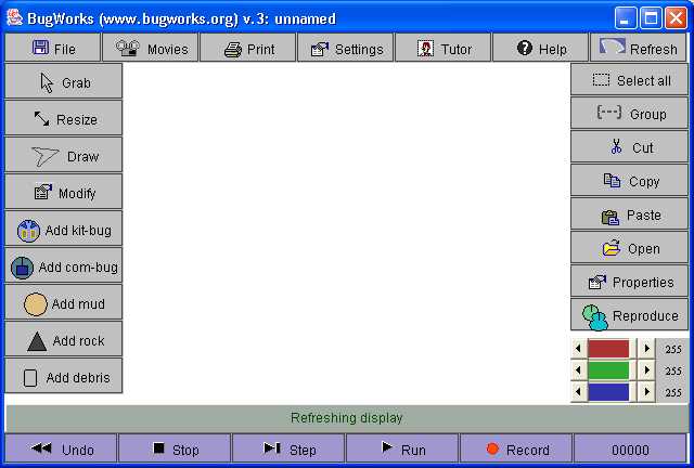
The main BugWorks window.
This is the main BugWorks display and work-area. The big
white area in the middle of the window is the `arena': this
is where you put your robots. Along the bottom are the
`tape transport' buttons, used for running the simulation.
The other buttons divide into three groups. Along the left
border are the tools, used mainly for adding robots and
other objects. Along the right edge are buttons for actions
applied to selected objects. Finally, there are buttons
along the top border for file operations, changing settings
and so forth.
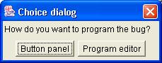
The com-bug dialog offers the option of two
control methods.
Choose `Program editor'. A new window will then be added,
which you should place somewhere below the main BugWorks
window. The new window should look like this:
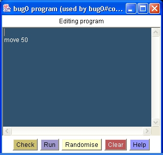
The com-bug window bug is a `program editor', used
for entering commands.
This is the bug's window. As a com-bug, the bug's behaviour
is controlled by commands and the window shows what those
commands are. It also allows you to add to and modify the
commands. This is why com-bug windows are sometimes called
`program editors'.
   move 100
   turn 90
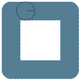
`First Box' (1 object, 104 frames) - A bug programmed to repeatedly execute a forwards
movement followed by a 90-degree turn builds up a square
pattern. In brackets are the number of objects involved in
the simulation and the number of cycles (frames) required
to build up the image.
Note the importance of pressing the `Show trails'
button! To generate BugArt, bugs *must leave a trail when
they move. But they will not do this until `Show trails'
has been pressed. Note also the slider next to the `Show
trails' button---only visible when the simulation is
running. This can be used to control the speed of the
simulation.
turn 45
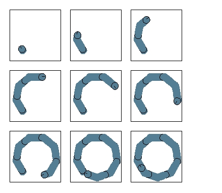
`First Octagon' (1 object, 130 frames) - Changing the angle of turn to 45 degrees builds up
an octagonal shape rather than a square one. Here the
build-up of the image is shown in a nine-part sequence which
runs left-to-right and top-to-bottom.
If you make the turn angle very small relative to the number
of steps taken, the bug will produce a circular pattern, as
in `First Circle'. As an experiment, try using
trial-and-error to work out how small the turn has to be in
order to achieve a visually smooth, circular trajectory.

`First Circle' (1 object, 480 frames) - Making the angle of turn small
converts the octagon-drawing bug into a circle-drawing bug.
In the present setup we have used a com-bug because these
are, in many ways, easier to control. But we can also
generate images using kit-bugs, added using the `Add
kit-bug' tool. The behaviour of these is more difficult to
manipulate. But they do have the advantage of having a
useful behaviour built-in. An unmodified com-bug just tries
to move forwards in whatever direction it is already
heading. An unmodified kit-bug on the other hand will
always try to move towards the nearest object in the arena,
whatever that object is. If you add two kit-bugs and set
the simulation running, the bugs will chase each other
around the arena. The generated image will be along the
lines of `First Chase'.
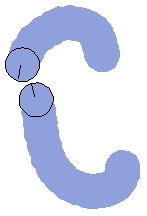
`First Chase' (2 objects, 21 frames) - Unmodified kit-bugs always try to move towards the
nearest object in the arena. If this is another bug of the
same type, the result is a mutual chase.
More information about controlling the behaviour of com-bugs
and kit-bugs will be provided later on.
Attribute changes
Images of circles and polygons can get boring. But it's easy
to liven things up. The trail left by a bug is a sequence of
impressions made by `stamping' its shape on the arena
surface. The bug's body shape and color are the `bricks'
from which the image is built up. So one way to change the
image is to change these attributes.
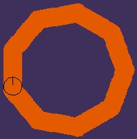
`Red Polygon' (1 object, 136 frames) - The color of the bug's body fixes the color of its
trail. With a red body color, we get a red pattern. With
nothing selected, moving the color sliders controls the
color of the arena.
An alternative way to change the bug's color is to use the
Properties dialog. In fact, this gives access to all the
attributes which you can change. For example, to change the
color of the body to yellow, open the Properties dialog,
pull down the color menu and select `yellow'.
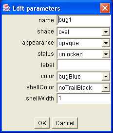
The Properties dialog gives access to an object's
main attributes.
In the Properties dialog you may notice that the bug's shell
color (the value of `shellColor') is given as
`noTrailBlack'. This is a special version of black which
doesn't show up in the trail.
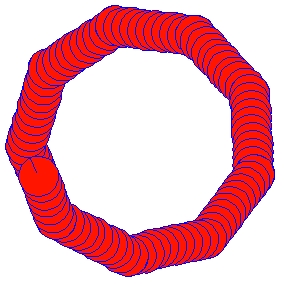
`Blue Shells' (1 object, 132 frames) - With a permanent shell color, a trail of shapes is
created. Colors whose names begin with `noTrail...' do not
show up in trails.
The special color `noTrailBlack' is used for all newly
created bugs. This is why borders do not normally appear in
trails.
Changing shape
The shape of the bug can also be changed using the
Properties dialog. BugWorks provides a range of built-in
shapes including `box', `triangle' and `oval'. There are
also some odd shapes such as `battery' and `chest'. To give
a bug a box shape, select the bug, open the Properties
dialog, pull down the shape menu and select `box'. With a
box-shaped bug we now obtain `Blue Box Shells'.
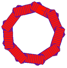
`Blue Box Shells' (1 object, 129 frames) - Using a red-brown, box-shaped bug and a program
combining a forwards move with a 40 degree turn, we get a
nine-sided figure. `Frills' at the corners result from the
way the bug stamps out a sequence of shapes as it turns.
Variations on this image can be generated by playing with
the attribute values. You can try different shapes, shell
widths, sizes and colors. But to obtain something really
new, we need to modify the underlying program of commands.
For example we might replace the existing program with the
following sequence of four commands:
   move 20
   turn -40
   move 20
   turn 80
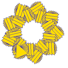
`Triangular Shells' (1 object, 179 frames) - A blue shell color and a triangular body makes the
most of this swivelling `gun-turret' action.
Creating new shapes
As well as letting you specify built-in shapes such as
`box' and `triangle', BugWorks also allows you to draw your
own shapes. For this you use the Draw tool from the main
window. To draw a new shape, select the Draw tool and click
somewhere in the arena. Each subsequent click will add a
new edge to the shape and you can continue adding edges as
long as you like.
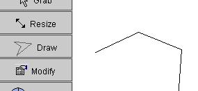
The Draw tool lets the user define new shapes by
clicking out a sequence of points in the arena.
When you've finished, click the mouse close to the starting
point. The system will finalise the shape and ask you to
provide a name for it. Once you've done this, the new shape
will be available for use in shape menus. `Beach Cutout'
shows the kind of shape that can be generated.
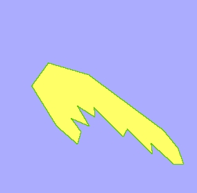
`Beach Cutout' (1 object, 39 frames) - A shape created using the Draw tool.
With a customised shape, new visual effects are easily
obtained. `Unstable Beach' was generated using the `Beach
Cutout' shape with a com-bug programmed to rotate on the
spot.
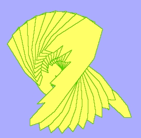
`Unstable Beach' (1 object, 39 frames) - With a hand-drawn shape even simple com-bug
programs may produce complex patterns.
Using the Resize tool, a bug with a custom shape may be
resized just like any other shape. Beware of making bugs too
large or too small. If you make a bug too small, you may
struggle to re-select it. If you make it too big you will
find that it is unable to do much within the confines of the
arena.
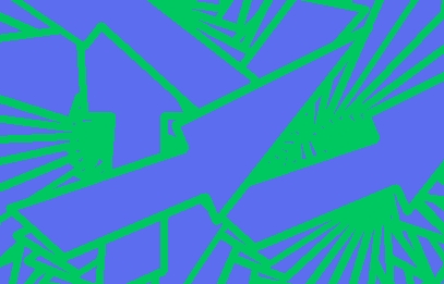
`Arrow Confusion' (7 objects, 15 frames) - The auto-swerving facility
creates endless rotation when bugs are too large to move
around within the arena.
All shapes, including the ones you draw yourself, can be
altered using simple editing methods. To edit a shape, click
on one of its corners to bring up the `drag handles'. You
can then drag any corner to a new position. If you wish,
new corners can be created by clicking over boundaries.
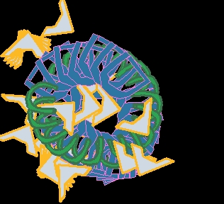
`Acdc' (3 objects, 27 frames) - An image created using letter-shaped, kit-bugs. All
the shapes used here were created using the Draw tool.
When working with shapes, you will find it easier
if you temporarily turn off `Show trails' and increase the
size of the object you are working on. With a larger object,
it is easier to bring up the grab-handles. It is also easier
to get the edits right. The size of the object can always be
reduced again when the shape has been finished.
![]()
Illustrating how a box shape can be turned into a
chevron shape by adding corners and dragging them to new
positions. (1) The original shape is a box. (2) Clicking on
a corner brings up the grab-handles. (3) A new corner is
made by clicking over the bottom edge. (4) A second corner
is made by clicking over the top edge. (5) The lower,
central handle is dragged upwards. (6) The upper, central
handle is dragged downwards.
Once a desired shape has been created, the Resize tool may be
used to stretch it widthways or lengthways. If you have not
previously given the shape a name, you can do this at any time
using the `ADD CHOICE...' option in the shape menu (from the
Properties dialog). Simply type in the name you want to use
and press OK. All shape menus will then include this shape as
an option. If you don't give a name to the new shape it will
be given a machine-generated name---something like `unnamed0'.
But do bear in mind that shapes will only be saved if you
save a simulation in which they are used. If you don't save
them this way, they will be discarded when you close the
system.
 move 100
 turn 90
 move 20
 turn 90
 move 100
 turn -90
 move 20
 turn -90
![]()
`Chevron Roller' (1 object, 666 frames) - The image illustrates use of a chevron shape with a
`roller action' program. The commands ensure that the bug
works its way across the image in a series of sweeps.
The program ensures that the bug moves back and forth
across the image, gradually filling in pattern. The
auto-swerving facility ensures that the bug is kept within
the arena's borders.
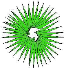
`Exploding Hook' (3 objects, 14 frames)
Changing colors and editing the shape to obtain a more
`whiskery' configuration produced the hairy-ball effect of
`Self Juggling Skittles'.
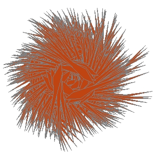
`Self Juggling Skittles' (4 objects, 167 frames)
Further illustrating the possibilities of shape editing,
`Hexplosion' was cast from a setup involving a single
kit-but whose original shape was `box'. One corner of the
shape was pulled out and a new one added along one of the
borders.
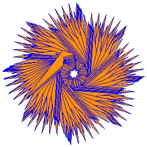
`Hexplosion' (1 object, 300 frames) - Two red-orange bugs rotate around a
central position. The pattern of collisions caused by the
knife-like bodies creates an explosive effect.
Programmed attribute changes
Com-bugs are mindlessly obedient agents. Once a particular
sequence of `move' and `turn' commands has been entered into
the relevant program editor, they will repeat the sequence
indefinitely, carving out a regular pattern across the
arena. But they can do much more than just move and turn.
There are a large number of commands which they will happily
obey; we will look at these towards the end of the book. One
command which is worth knowing from the outset, however, is
`set'. This can be used to make the bug change its
appearance. For example, to have the bug change its color to
red, you would use a `set' command like this:
set bug.color = red
set bug.shape = box
set bug.shellColor = invisible
   set bug.width = 25
   set bug.length = 50
   set bug.shape = triangle
  set bug.width = 19
  move 6
  set bug.shellColor = randomColor
  set bug.shellWidth = 4
  set bug.heading = 159
  turn 169
  set bug.color = randomColor
  set bug.width = 18
  turn 162
  move 7
  set bug.shape = box
  move 14
  turn -102
  set bug.heading = 251
  turn 148
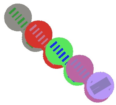
`In Training' (1 object, 317 frames) - An unusually well-organised image cast from a
simulation using a single, randomly-programmed com-bug.
Pause
Using the basic tools introduced in this chapter---the `set',
`move' and `turn' commands, shape-drawing, attribute changes
etc.---you should now be equipped for some self-motivated
experimentation. If your initial efforts tend to produce
nothing very unimpressive, do not give up. As with any
creative endeavour, BugArt requires perseverance. You may
have to go back and re-read bits of the text several times
before things become clear. When it comes to manipulating your
bugs, you'll find that they almost certainly will not do
what you expect first time around. But whatever they do do,
there will a logical reason for it. And however much it may
seem that they are deliberately trying to be difficult, this is
just an illusion!
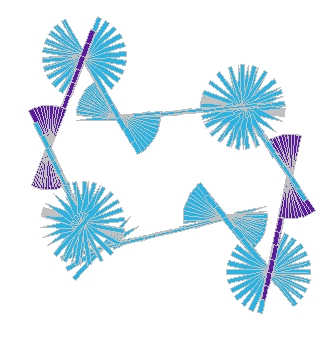
`Twizzles' (1 object, 340 frames) - In this image a chrystaline effect is
achieved using an elongated bug that repeatedly executes a
rotational movement followed by a forwards transition of a
fixed length. `set' commands were used to give the bug a
cyan color during the full rotation but a more violet shade
during the semi-rotation. The general effect is cold and
wintry, reminiscent of patterns of frozen condensation.
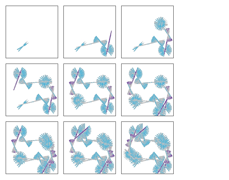
`Twizzles' (1 object, 340 frames) - This is the `Twizzles' image shown as a nine-cell
cast-grid. The cells show the accumulation of trails over
nine, equal intervals.
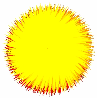
`Supernova' (2 objects, 775 frames) - This image, which features the rotation
of a hand-drawn bug, demonstrates how the underlying
`buginess' of the image-creation process can be masked by
accumulated trails.
In many cases, an image will make use of a short simulation
sequence, i.e., a brief spurt of behaviour. In other cases,
the image is built-up over a larger number of cycles. In
some cases images may require a considerable length of
simulation. `Firewheel' is a case in point. This requires
several thousand simulation cycles to reach the desired
state.
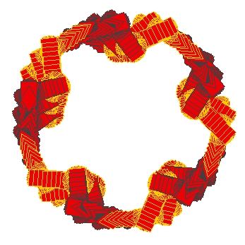
`Firewheel' (1 object, 3219 frames) - Here a braiding effect has been
achieved using a single bug moving in a fixed cycle. The
reds and golds are introduced by explicit color-change
commands applied while the bug is in motion.
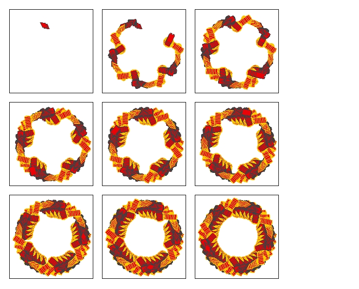
`Firewheel' (1 object, 3219 frames) - The same image, shown as a cast-grid.
In traditional art, the artist controls a small number of
variables---principally the color and shape of marks being
made. In BugArt, the artist has access to a much wider range
of variables. When using a com-bug, for example, there will
be a sequence of `set', `move' and `turn' commands to
conjure with. Changing any one of these will affect the
image. Each command is effectively a variable under the
artist's control.
The Modify window
BugWorks provides a range of mechanisms for `creativity
support'. Of these, the most useful is probably the Modify
window. This allows multiple attributes of objects to be
changed `all in one go'. It is a kind of labour-saving device
for bugartistes.
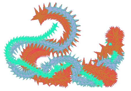
`Star Salute' (3 objects, 260 frames)
Where we have more than two bugs, the dynamics of the
simulation may be more difficult to predict. Each bug
attempts to move towards the nearest object but this may
change from moment to moment. The interactions that can
result can be difficult to predict and quite good visual
results can be generated using a large number of
different-looking kit-bugs. This is where the Modify window
comes in handy. It makes it easy to randomise the visual
attributes for a set of bugs using a single button-press.
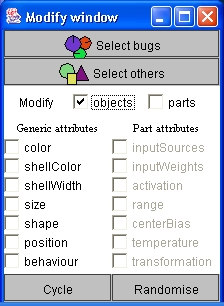
The Modify window is used to modify multiple
attributes all in one go.
The Modify window needs to be placed somewhere below the
main window, as in this typical layout for a BugWorks
session:
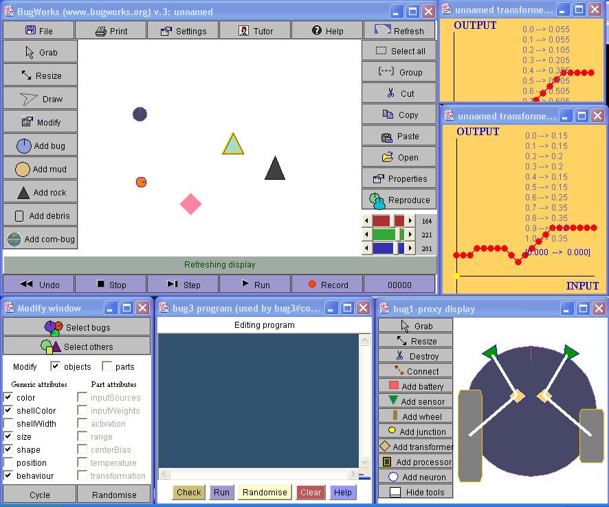
A possible layout for a BugWorks session. The
screenshot shows the main window along with several bug
windows, the Modify window and a selection of part windows.
Use the `Select bugs' button from the Modify window to
select all the kit-bugs you have added to the arena. Then
tick the `color' check-box. You can now use the Cycle
button to change the color attribute of all the bugs in the
simulation with a single button press. Each time you press
Cycle, all the bugs will be given a new color in a
pre-defined sequence. This looks more interesting if you
try it with the simulation running. The effect will be
something along the lines of `Stariation'.
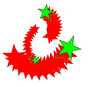
`Stariation' (3 objects, 26 frames) - Using the Cycle button from the Modify window, the
colors of all the bugs in the simulation can be changed
simultaneously.
Instead of Cycle, you can use the Randomise button to set each
selected bug to have a randomly selected color. To find the
best color combinations for the current simulation, simply
press the Run button and keep pressing the Randomise button
until you achieve a satisfactory effect. `Mace Eye' is a
typical result. It was constructed from the simulation used to
generate `Star Salute' after the randomisation facility had
been used to modify sizes, colors and shell colors.
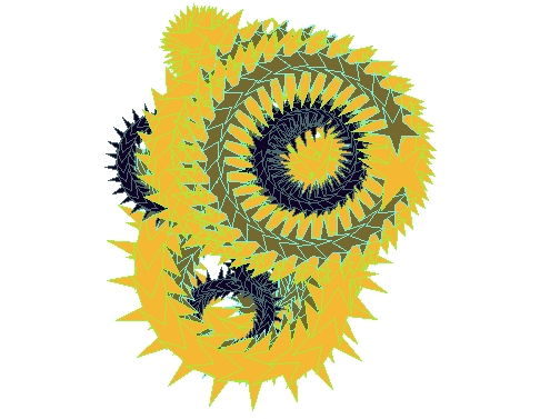
`Mace Eye' (3 objects, 482 frames) - The Randomise button from the Modify window is
useful for exploring attribute combinations.
The Modify window lets you randomise or cycle any attribute
you like. But for now, leave the `appearance' and `parts'
check-boxes unticked. Use of these options involves involves
knowing something about the innards of bugs---a topic we will
look at later on.
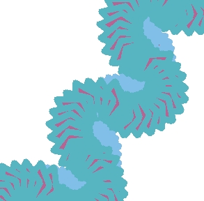
`Pleasant Thoughts' (2 objects, 150 frames) - Demonstrating the effect of using a high
shell-width value, this makes use of a com-bug programmed to
execute a `wriggling' motion.
The image `Angry Thoughts' on the other hand was generated
from the same bugs running in the same simulation, but with
shell widths set to the normal value 1. It is also possible
to set the `shellWidth' value to 0 in order to eliminate
shells completely. (Another way to achieve the same effect
is to set the `shellColor' to `invisible'.)
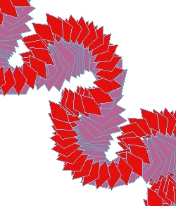
`Angry Thoughts' (2 objects, 156 frames)
Use of extremely high shell width values, together with spiky
shapes (such as a star shape) can produce very blobby
patterns, as in `Thick Star Shells'. This is one way to
break-up unwanted `geometricality'.
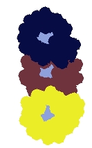
`Thick Star Shells' (4 objects, 4 frames) - This image, cast from a very short sequence of a
simulation, shows three star-shaped objects all of which
have been given a large `shellWidth' value.
When used in conjunction with a small group of kit-bugs,
the Modify window is capable of generating more or less
endless visual variety, particularly when the Randomise
button is used to manipulate multiple attributes. `No Room
in the Basket', for example, was derived from `Thick Star
Shells' using just a few clicks of the Randomise button.
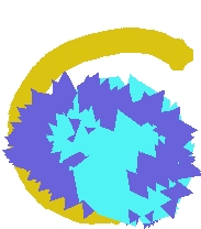
`No Room In The Basket' (3 objects, 58 frames)
Commonly, experiments using the Modify window begin with
all bugs and all generic attributes selected. The Randomise
button is then utilised until one of the bugs acquires an
interesting appearance. This is then de-selected,
effectively protecting it from subsequent modification.
Further randomisation can then be applied to try to enhance
the appearance of the remaining bugs. This process of
incremental refinement can also involve the progressive
de-selection of attributes.
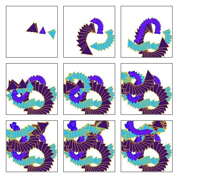
`Dragon Tails' (3 objects, 103 frames) - The cast-grid shows how even a simple simulation
rapidly `clutters up'.
As you can see, images constructed using multiple bugs can
become cluttered very quickly. The best looking frames often
occur early on in any simulation run, as is illustrated in
this cast from a short initial sequence of `Dragon Tails'.
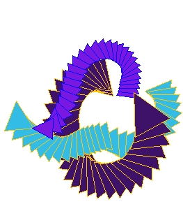
`Dragon Tails' (3 objects, 103 frames) - This image was cast from a short,
initial sequence of the `Dragon Tails' simulation. With
greater levels of complexity, less is often more: an image
generated from a shorter sequence will often pack a
stronger visual punch.
Red-green-blue (RGB) values and ranges
After the Randomise or Cycle button has been used to update
attribute values, you may find it useful to open a
Properties dialog to see what the new attribute values
actually are. In most cases, the new values should be
self-explanatory, e.g., the shape attribute may have changed
from `oval' to `triangle'. But changes made to `color' and
`shellColor' attributes may need interpretation.
0 180 255

255 0 0
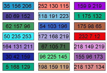
Color samples with their corresponding RGB
(red-green-blue) specifications. The first number in each
sequence specifies the red intensity, the second number the
green intensity and the third the blue intensity.
When using the Cycle button to change color attributes,
color values will be reset to standard color names. However,
when using the Randomise button, color values will be set
to RGB values. This helps to maximise diversity. (There are
many more possible RGB values than there are named colors.)
Randomisation ranges
BugWorks allows you to control the range from which random
colors are selected via the setting of `randomColorRange'.
In the Settings dialog (accessed from the main window) you
will find this is initially
0-255 0-255 0-255
0-100 0-100 0-100
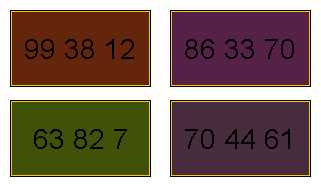
Colors randomly generated using the
`randomColorRange' value `0-100 0-100 0-100'.
If you change the `randomColorRange' to
0-255 0 0
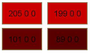
Examples of colors randomly generated using the
scheme `0-255 0 0'.
If you want colors to be lightened shades of magenta, say,
you would have to specify something like
255 0-255 255
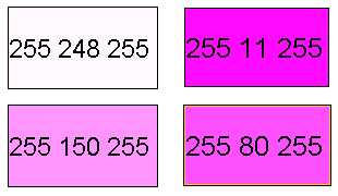
Examples of colors randomly generated in the scheme
`255 0-255 255'.
In contrast, the value
255 255 0-255
0-255 R R
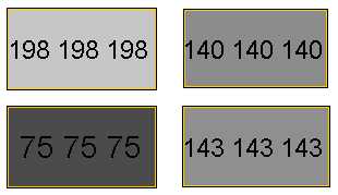
Shades of grey generated randomly using the scheme
`0-255 R R'.
For even greater control you can use symbolic expressions
like `R/2' and `G+30'. For example, the specification
G 100-200 G-50
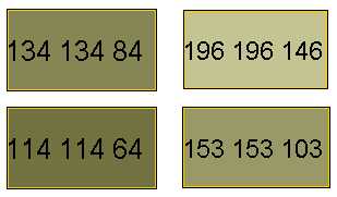
Colors generated using the spec `G 100-200 G-50'.
It is also possible to use multiplication and division. This
can be a convenient way to maintain the same color `percept'
over a number of shades. For example, use of the scheme
B*2 B+40 80-100
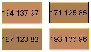
Colors generated using a spec featuring
multiplication and division.
One final example!
200-255 R/2 90
Program randomisation
Randomisation is a powerful tool in BugArt because it
enables the image-maker to harness the power of
trial-and-error. When randomisation is implemented via the
Modify window, the effect may be distributed across any
number of objects. Trial changes can then be applied to any
number of attributes in any number number of objects.
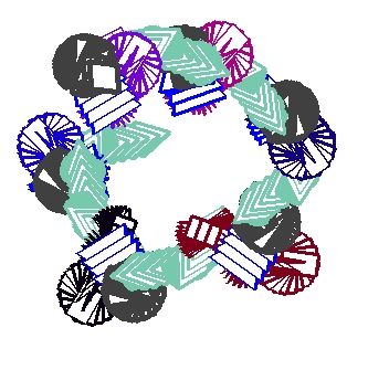
`Beserker' (1 object, 900 frames)
Program randomisation will occasionally generate
interesting structures involving interleaved patterns of
repetition and translation. `Unwashed Blanket' is a good
example as is `Illogical Tool'.
![]()
`Unwashed Blanket' (1 object, 1235 frames)
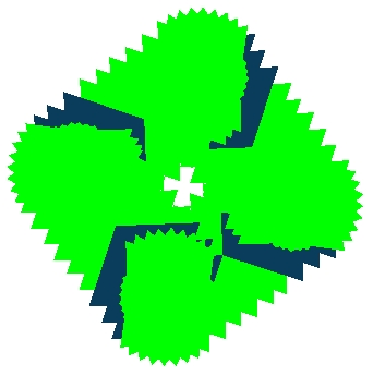
`Illogical Tool' (1 object, 81 frames)
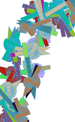
`Depression With Holes' (4 objects, 108 frames) - Illustrating the effect of program re-use, this was
cast from a simulation involving a group of four bugs all
executing the same steps in sequence, but at different
locations and headings.
Another example is `Hole in the Plan'. This used three,
identically programmed com-bugs. The commonality in behaviour
here produces a striking regularity.
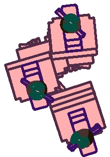
`Hole In The Plan' (3 objects, 384 frames) - This image was cast from a
simulation featuring a group of bugs all following the same
sequence of commands. The sense of lopsided symmetry results
from the duplication of behaviour at different locations and
orientations.
Using random values in commands
Randomisation can also be achieved by inserting `random'
values into commands themselves. For instance, it is
possible to use the command
move random7
turn random90
set bug.color = random255 random255 random255
set bug.color = random255 random80 random80
set bug.shellColorB = random255
set bug.color = 200 + random55
set bug.color = randomColor
set bug.shellWidth = randomShellWidth
Behavioural cycles
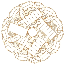
`Petallic' (1 object, 439 frames)
Commands using random turns or moves are a useful way of
injecting diversity and ensuring that the behaviour does not
fall into a repeating cycle. When random moves and turns are
implemented, the bug's behaviour will be more along the lines
of a `random walk' through the arena. For example, a single
com-bug using the program
  move 10
  turn random100
  move 10
  turn -random100
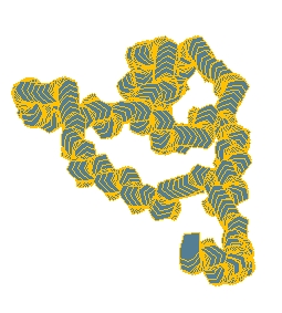
`Random Twisting' (1 object, 879 frames) - A simple random-walk through the arena.
Random walks are a good way to fill in a large area of
texture, as can be seen in `Group Ladder Scribbling', which
features several com-bugs running identical programs
containing random moves/turns.
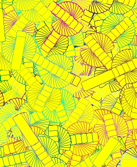
`Group Ladder Scribbling' (6 objects, 724 frames) - This image illustrates the way in which random
walks can be used to fill the arena with pattern.
`Snakes and Ladders', generated from a similar setup, shows
some unusual chain effects, resulting from the use of
invisible bodies in certain parts of the simulation.
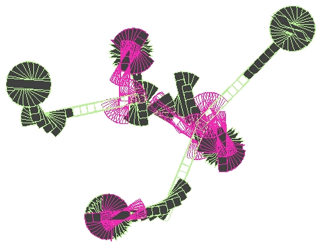
`Snakes And Ladders' (3 objects, 300 frames) - This image was developed using three com-bugs
running the same program. The laddering results from the
way in which bodies are made invisible for a part of the
sequence. Only the shell of the bug is then drawn, allowing
other image detail to show through.
Bug sex
As a final support for randomisation, BugWorks provides the
possibility for `sexual reproduction', or at least a BugArt
version of it. This is provided via the Reproduce button on
the right of the main window. Pressing this button will
generate a `mutant offspring' from whatever bugs are
currently selected. If two bugs are selected when the button
is pressed, the process is performed in a manner
reminiscent of sexual reproduction in nature. The offspring
is generated by creating a new bug which inherits attributes
from both parents, with a small element of randomisation
thrown in. If a single bug is selected when the button is
pressed, the process is carried out in a manner which mimics
asexual reproduction. The offspring is simply a mutated copy
of the parent.
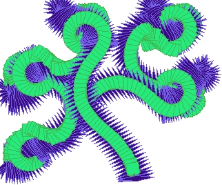
`Hand Of Hooks' (2 objects, 532 frames) - Changing bug shape produces subtle
modulations in the tail-chasing antics of kit-bugs. In this
image, a distended diamond shape, derived using the
Reproduce button, paves the way for a novel, hooking motion.
Pause
In a procedure known as `The British Museum Algorithm', 100
monkeys typing randomly on 100 typewriters eventually
produce the Complete Works of William Shakespeare. The
algorithm is known to be feasible in principle. But, of
course, it could never be completed in practice due to the
huge amount of time required (longer than the age of the
universe). This result is often taken as demonstrating that
random processes cannot play any real role in creativity.
And it might be thought to throw doubt on the validity of
some of the techniques described in this chapter.

`Paint It Mauve' (3 objects, 656 frames)
`Paint it Mauve' was constructed using three com-bugs and
the `roller' command sequence used earlier for `Chevron
Roller'. The bugs were given invisible shells and random
body colors with `randomColorRange' set to
B-100 B-50 150-255
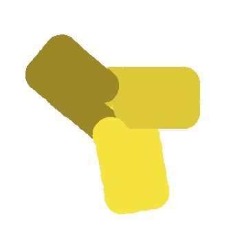
`Paint It Yellow' (3 objects, 48 frames)
Random colors chosen from these ranges will have a fairly
high red value (in the range 150-255), a green value that is
just slightly less then the red value and a blue value that
is the red value divided by 4. Such colors tend to be a
muddy yellow/brown.
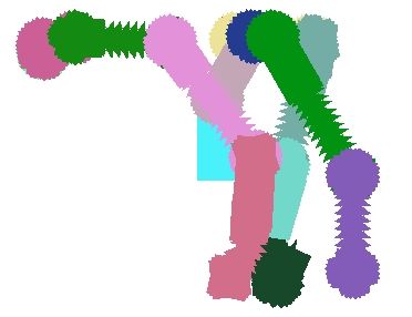
`Walker' (3 objects, 152 frames) - Illustrating the use of duplicated com-bug programs
derived using the Randomise facility of the program editor.

`Headache' (2 objects, 23 frames)
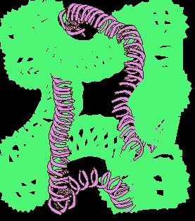
`Keep Off The Beanstalk' (2 objects, 153 frames)
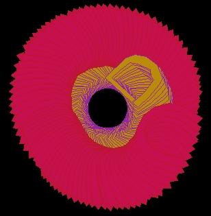
`Cool Deviance' (2 objects, 95 frames)
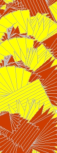
The quick and easy way to create BugArt involves using a
printer. First you create your simulation. Then you press
Run and switch trails on. After a while you stop the
simulation, press Print and the generated image pops out of
your printer.
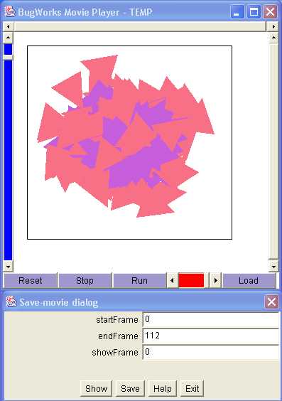
Recorded simulations may be saved as movies using
the Save-movie dialog in conjunction with the movie-player.
The basic usage of this facility should be self-explanatory.
To review the recorded movie, press the Run button in the
movie player, or simply click somewhere in the window. To
save the movie to disk, press the Save button in the dialog.
The show frame
Casting an image from a movie involves inserting an
appropriate value for the `showFrame' field in the
Save-movie dialog. This value specifies how far the movie
should be advanced when displayed as a static image. By
default, the value is zero, which means that only the first
frame is displayed. By changing the setting, we can
arrange for the image to show the accumulated trails from
any amount of initial `footage'.
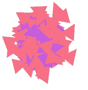
`Cracking Up' (2 objects, 193 frames)
In making the cast, the movie was first advanced to frame 8.
At this point the movie player window looked like this. Note
the 8 appearing in the top, left corner.
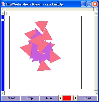
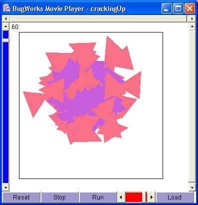
Setting endFrame and startFrame values
Before saving the movie you can also change the settings
for `endFrame' and `startFrame' if you wish. These define
where the movie starts and ends. Changing the `startFrame'
setting may be useful if the movie features some unwanted
footage right at the start. Changing the `endFrame'
setting, only affects the movie when it is displayed as a
`cast-grid' (see below).
The zoom setting
The zoom facility provides another way to control what appears
in the image. To zoom in on a region of the arena, use the
selection-box, i.e., drag the pointer across the relevant
area. The window will automatically reconfigure to display
just the selected region. To reset the zoom level,
double-click the window. Zooming can also be done using the
left-hand scroll-bar.
Casting example
As an illustration of what can be achieved through casting,
consider the two images below. Both of these were derived
from the same movie, which was itself derived from a
simulation involving three skittle-shaped kit-bugs.
`Hexplosion' was produced directly from the saved movie,
without any zoom being applied and without changing the
`startFrame' value. The `showFrame' was set to the final
frame of the movie (i.e., the `endFrame' value) so as to
ensure that the image would contain the entire accumulation
of trails.
`Hexplosion' (1 object, 300 frames)
Contrasting with this, we have `Hole in the Hex'. This was
cast from the same movie using a zoom setting focussing on a
small central region of the arena and a reduced `showFrame'
value. By focussing on a small region of the arena and a
shorter sequence, the cast yields a very different image.
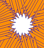
`Hole In The Hex' (1 object, 260 frames) - A contractive cast focussing on a small central
region of the arena.
Cast-grids
Setting the `showFrame' value to an early frame in a
simulation sequence produces a `snapshot' of the activity
that occurs up to that point. Chained together in a
sequence, such snapshots provide a static representation of
how the movie progresses over time. Snapshot chains like
these are called `cast-grids'---several examples have
already been seen in previous chapters. The image
`firstOctagon' is shown in cast-grid form, for example, as
is `Twizzles'.
Pause
Casting images from movies may seem like a slightly exotic way
of creating static images. But in a sense, the process is just
an extension of the traditional process of framing. The
placement of different borders around an image can have a
dramatic effect on the image's visual impact. Traditional
artists therefore take steps to ensure that their images are
given the right frame before being displayed. But for
traditional art, framing is essentially a `post-production'
issue, something to be considered after the original image
has been completed. The creative process should be completed
before the framing process begins. Were the latter to
influence the former, it would be the `tail wagging the dog.'
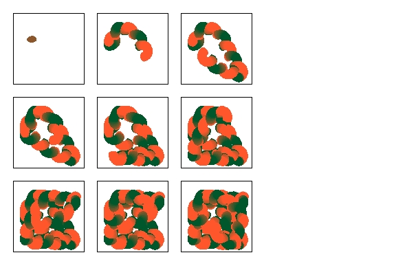
`Curry Aftermath Pre Cast' (1 object, 1919 frames) - A neutral cast-grid representation drawn from a
simulation involving a single com-bug executing a lurching
motion with color-change effects.
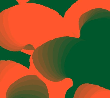
`Curry Aftermath' (1 object, 1919 frames) - A cast utilising a narrow zoom setting so as to
focus on a small region of the arena. The image benefits
from the removal of extraneous white space around the edge.
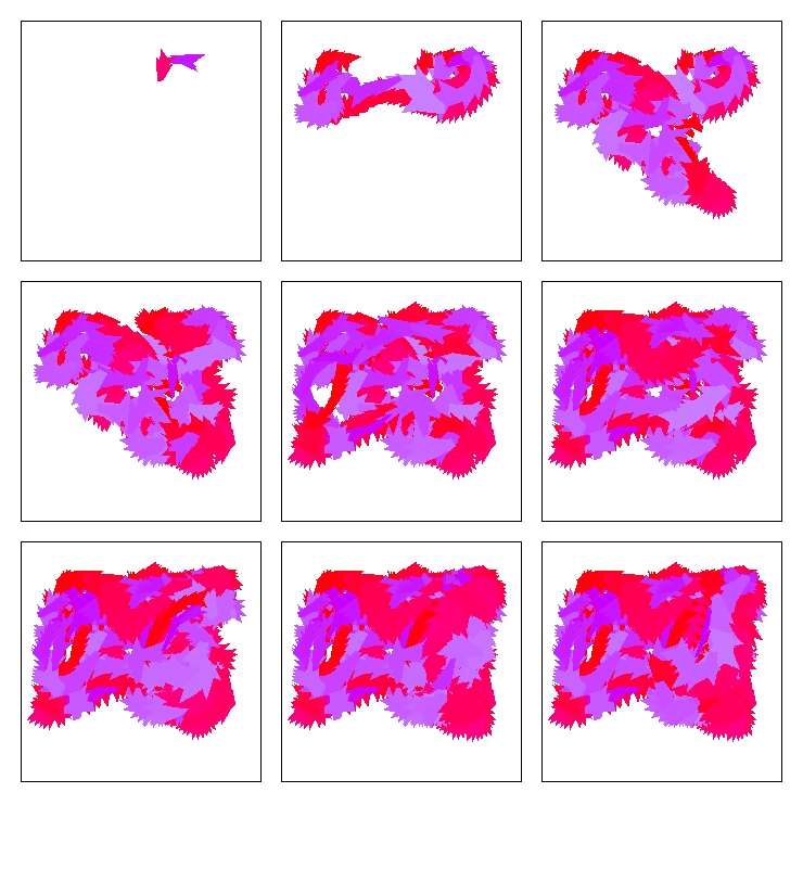
`Bad Head Pre Cast' (2 objects, 595 frames) - In this neutral cast-grid presentation, trails
created by the bugs in the simulation only partially cover
the arena.
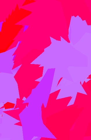
`Bad Head' (2 objects, 595 frames) - A cast isolating a fully-covered region from the
right half of the arena.
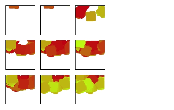
`Prozac' (6 objects, 276 frames) - The original simulation paints color into a small
area of the arena.
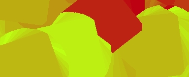
`Prozac' (6 objects, 276 frames) - In this cast, the image is rendered without any
`gaps'.
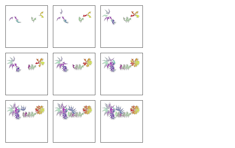
`Emotional Cricket' (8 objects, 29 frames) - Trails from the original simulation are mainly
focussed in the top half of the arena.
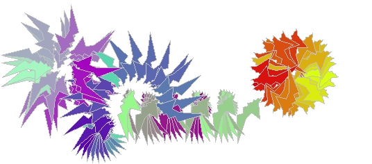
`Emotional Cricket' (8 objects, 29 frames) - In this cast, the zoom level has been set so as to
neatly frame the filled portion of the arena.
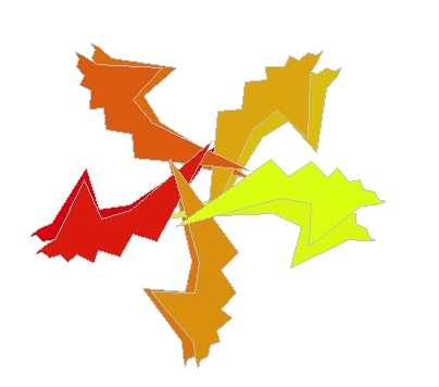
`Emotional Cricket Cast2' (8 objects, 29 frames) - This highly contractive cast samples just the first
ten frames of the construction of the the ball pattern on
the left.
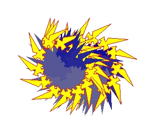
`Two Towers' (2 objects, 110 frames)
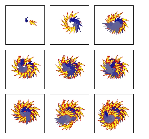
`Two Towers' (2 objects, 110 frames) - A cast-grid representation in which the grid
layout appears to add visual interest to the underlying
image.
The behaviour of a com-bug is the result of its program of
commands. But with kit-bugs, it is the components and the way
they are wired up that makes the difference. Opening a window
onto a kit-bug will clarify what this means. Examining the way
the internal components of the kit-bug are organised will show
why an unmodified kit-bug will always tend to move towards the
nearest object.
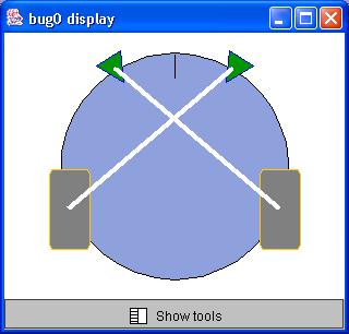
A kit-bug's window. The two sensors are shown as
green triangles while the wheels are shown as grey
rectangles. Note the way each sensor makes a connection to
the wheel on the opposite side. It is this
`cross-connection' which causes stimulation to flow to the
opposite side of the bug. This ensures that the bug always
moves towards the stimulus rather than away from it.
You will see the circular body of the bug with its `nose
line' pointing upwards. In the lower half of the window
there should be a couple of gray, box-shaped components.
These represent the wheels. In the top half, there should be
a couple of triangular components. These represent the
sensors. All of the objects in the window can be dragged
around using the mouse.
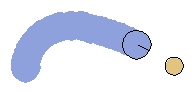
`Simple Approach' (2 objects, 18 frames) - A cross-wired bug will always tend
to turn and move towards the closest stimulus. The rate of
turn is highest when the bug is side-on to the stimulus.
Another appealing property of the cross-wired bug is that it
is easy to modify its dynamic properties. The rate at which
the bug turns towards any sensed object depends on the
difference between the two sensor signals, which in turn
depends on the difference in the position of the sensors
relative to the object in question. To obtain faster turns,
we only have to move the sensors further apart. To obtain
more gradual turns, we shift them closer together. The idea
is illustrated in the screen-show below. It shows two bugs
in plan view, one with sensors set wide apart and the other
with them set closer together.
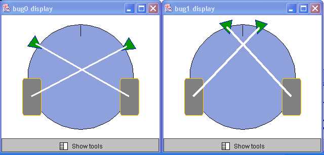
By moving sensors
further apart, the difference between
sensor-to-object distances is increased. The
result is that there will be a greater difference in
the speed of the two wheels and the bug will tend to
turn more quickly towards the closest object.
The difference that sensor separation makes on behaviour is
illustrated in `Different Curves'. This shows how three,
differently configured bugs move towards a small yellow
target in the bottom, left corner of the arena. The image
was created by setting up three kit-bugs each with a
slightly different degree of separation between its sensors.
The bug with widely spaced sensors turns quickly towards the
object while the other two turn more slowly. The bug whose
sensors are very close together only turns very slowly
towards the target.
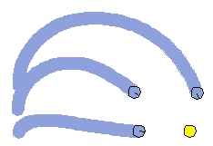
`Different Curves' (4 objects, 141 frames)
(If you are wondering why the three bugs in `Different
Curves' do not try to turn towards each other, it is
because they were configured to use filtered sensors.
The way these work is described later on.)
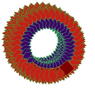
`Basic Chase' (3 objects, 460 frames) - The chase effect obtained from
kit-bugs is more interesting with randomised color, shape
and size values. Here the two bugs pursue each other in a
race-track pattern which gradually shifts downwards and to
the right, creating a 3-dimensional effect.
As ever, judicious use of the Modify window to vary
properties such as color, shape and size will quickly
produce very different looking results.
Other parts
Kit-bugs may have any number of parts and these can be
connected together in any number of ways. There are several
different types of part in addition to sensors and wheels.
Changing a bug's configuration of internal parts changes its
behaviour. But often the change will be hard to predict.
Using component trails
Aside from being a way of manipulating behaviour, the
introduction of parts is an interesting way to vary a bug's
`paintbrush' characteristics. After the `appearance'
attribute has been set to `transparent' in the Properties
dialog, a bug's internal components will be visible, just
as they are in the Open window. This means they will show
up in the trail. With its parts on display, the trail made
by a bug becomes considerably more detailed. Since it is
possible to modify a part's attributes (size, shape, color
etc.) in the same way as one modifies those of a bug, these
part trails can be used to create a range of visual
effects.
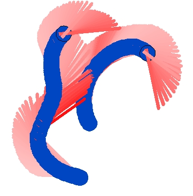
`Wormingoes' (16 objects, 127 frames) - An image in which sensor-motor
connections protrude outside the body of the host bug. The
coloration effects result from the way in which the system
uses shades of red to display the amount of signal being
carried on a connection.
`Peeping Pink' is from the same setup. Generated using
kit-bugs and the default activation colors, sensors
were again pulled well out from the body and all parts were
made invisible.
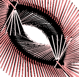
`Peeping Pink' (18 objects, 117 frames) - Another image exploiting protruding parts. Here the
striation effects created by the sensor-wheel channels
dominate the layout.
When exploiting channel coloring in this way, it may be
helpful to use larger channels. This can be achieved by
modifying the value of `channelWidth' in the Properties
dialog. With a larger `channelWidth' value, the channel
coloration effects will stand out more strongly. For maximum
impact, lose the bugs altogether by selecting `invisible'
for both body and shell color. `Bashful Alien' is a version
of `Wormingoes' which exploits invisibility in this way.
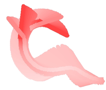
`Bashful Alien' (8 objects, 150 frames) - Simulation possibilities are
pushed to the limit in this image, which is built up solely
from the coloration effects applied to sensor-motor
connections of two invisible bugs.
All the color conventions can be altered in the settings
dialog. The way signal levels are represented is defined by
the setting of `activationColorRange', which works in much the
same way as the `randomColorRange' setting. Normally, this is
set to
255 0-255 0-255
255 0 0
255 255 255
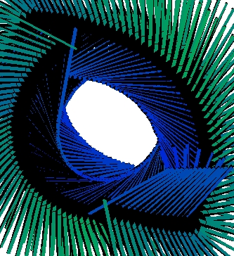
`Peeping Blue And Green' (18 objects, 110 frames) - Also cast from the `Peeping Pink' setup, this
makes use of a green/blue color scheme for channel colors.
Using `140 140 0-255' for `activationColorRange' with the
same setup used for `Bashful Alien' produces the
differently flavoured `Bad Air Day'.
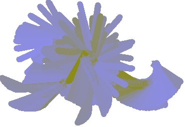
`Bad Air Day' (8 objects, 100 frames) - Here the channel color scheme constrains red and
green intensities to a single value, effectively forcing all
the color variation to be expressed through the blue
intensity.
(If you want to experiment with activation-color ranges,
you can specify the word `random' as the setting
for `activationColorRange' and the system will then
automatically choose a random setting for you.)
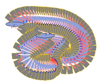
`Zipper Knot' (14 objects, 45 frames) - An image generated using two
transparent, cross-wired bugs. In each bug, the wheels were
enlarged and moved slightly apart and the left-hand sensor
was relocated to the lower, left quadrant of the bug.
When experimenting with transparent bugs, it is often
desirable to modify properties of the parts of all the
bugs in the arena. This is the sort of task for which the
Modify window is well suited. To randomise the shapes of
all the parts of a set of bugs, first select all the bugs to
be modified. Then open the Modify window and tick the
`Parts' checkbox and the `shape' checkbox. Pressing the
Randomise button will now randomise the shapes of all the
parts of all the selected bugs. `Zipper Twist' exemplifies
what can be achieved.
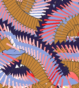
`Zipper Twist' (14 objects, 167 frames)
Remember that any shape with corners can be edited. This
applies equally well to parts. If the randomisation of part
shapes has produced a shape with corners, it is possible to
modify that shape by (a) clicking on a corner to bring up
the grab-handles and then (b) pulling the handles to
whatever position is desired. `Zipper Slasher' and `Zipper
Hog'
were produced by pulling out the apex of the triangular
shape of the left wheel, prior to re-running the simulation.
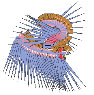
`Zipper Slasher' (14 objects, 36 frames) - the cold, blue spikes scything
across the image result from the use of an elongated
triangle for one of the bug's sensors.
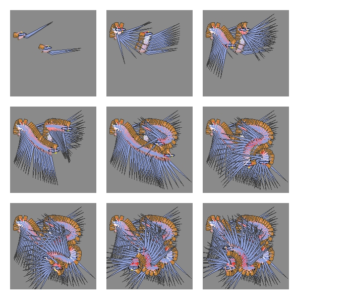
`Zipper Hog' (14 objects, 104 frames) - The blood-red splashes in the centre
of the image result from bursts of activity on sensor-wheel
channels.
Still more extreme effects can be obtained by using the Modify
window to randomise `inputSources', an attribute of all parts.
This attribute defines which other components have a
connection in to the part. By randomising its value, one is
effectively reconfiguring the internal configuration of the
bug with a single button push. Surgery on the cheap!
Bug dynamics
As noted, the standard kit-bug is `cross-wired'.
The sensor on one side of the bug drives the wheel on the
other side with the effect that the bug always turns towards
whatever is closest to it. But the sensor-motor connections
may also be uncrossed. In other words, they can be set so
that the left sensor drives the left wheel and right sensor
drives the right wheel. The behaviour produced by the bug
then changes in an interesting way. Rather than approach the
closest object, the bug will now try to move away from it.
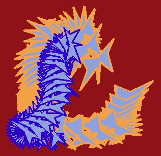
`Pester Power' (2 objects, 63 frames) - Kit-bugs are easily re-configured so as to exhibit
`evasion'. In this case, they always attempt to move away
from the nearest object.
`Pester Power' provides a simple demonstration of the
effect. Two standard, kit-bugs are involved, both using a
custom shape and an enlarged shell width. The sensor-wheel
connections in the larger bug have been uncrossed with the
result that it responds by trying to move away from the
smaller bug. A deep red background has been used here for
maximum color contrast.
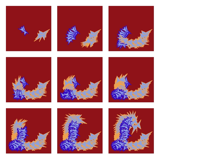
`Pester Power' (2 objects, 63 frames) - Due to different internal
configurations, the two bugs here display opposite
behaviours. The smaller bug repeatedly tries to approach the
larger bug, while the larger bug attempts to move away.
With cross-wired bugs, the strength of response depends
largely on the separation of the sensors and the size of the
wheels, which is itself affected by the size of the bug.
Bigger wheels produce more speed and if wheel-size is
increased substantially, the bug will appear to `jump' from
position to position. This can produce scatter effects, as
in `Evergreen'. The image was generated using two
ant-shaped, kit-bugs one of which was equipped with
extremely large wheels.
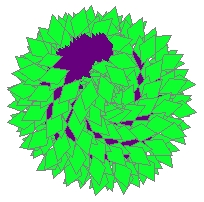
`Evergreen' (2 objects, 197 frames) - Giving a bug oversized wheels enables
it to `jump' from position to position. In this setup, the
wheels for the green bug were made large while the wheels
for the purple bug were kept small. The result is that the
green bug circles the purple bug, moving forwards in large
jumps.
Where bugs travel smoothly around the arena, the visual
effect will always be somewhat `tubular'. Giving bugs the
ability to jump can thus be a useful way of injecting
novelty. Expanding wheel length is a quick and easy way to
produce jumping. But there are other ways to do it.
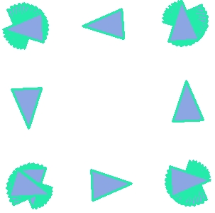
`Niner' (1 object, 46 frames)
`Cubism' exploits a different form of jumping. All the bugs in
this setup are kit-bugs with rectangular bodies and invisible
shells. Normally they would travel smoothly around the arena.
However, because the global setting for `gridCellSize' has
been increased from 1 to 10, the bugs are effectively being
`snapped to grid' each time a move takes place. With a cell
size of 10, the grid is very coarse grained (i.e., large
cells). The result is that the bugs are compelled to jump from
position to position, rather than moving smoothly between
them. Normally, the `gridCellSize' setting is used as a means
of facilitating more precise location of objects by hand. But
like everything else in the system, it can be pressed into
service as a way of conjuring up novelty.
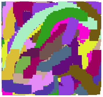
`Cubism' (16 objects, 210 frames) - A complex image constructed from simple
components. Fifteen rectangular, kit-bugs execute a mutual
chase. But the imposition of of a coarse-grained grid on the
arena (via the setting of `gridCellSize') forces bugs to
jump from position to position.
Pause
Illustrating some of the ways in which the techniques
described in this chapter can be put to use, the pause gallery
for this chapter presents a range of images constructed using
transparent bugs, i.e., bugs with their parts on show. Various
other techniques from preceding chapters have been brought
into play at the same time.
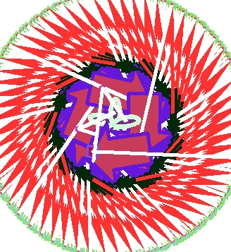
`Visit From James' (11 objects, 195 frames) - Two arrow-shaped bugs execute a tight, mutual
chase. The pulled-out sensors set up a vortex of
interlocking bars.
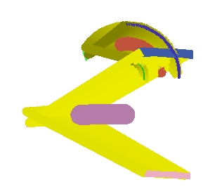
`The Future Is Yellow' (14 objects, 65 frames) - An unusual offering, cast from a simulation
involving two kits bugs with massively enlarged channels and
a `activationColorRange' value producing shades of yellow.
Demonstrating, if nothing else, that not all BugArt is
spirographic.
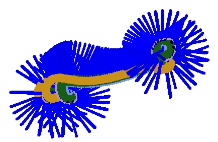
`Billipede' (8 objects, 183 frames) - Enlarged and protuding channels are again used to
generate dynamic linear effects. A blue scheme has been used
here for displaying channel activation.
In traditional art, the quality of the image is not only a
result of the marks made. The surface on which the marks are
made also influences the result. Different surfaces yield
different effects and traditional artists may go to great
lengths to ensure that a surface's properties are exactly
right.
Use of these objects in BugArt involves taking advantage of
the way in which they modulate interactions with bugs.
Getting stuck into mud
Rock objects can be put to use as attractors for guiding
bugs along desired trajectories. Used carefully, they can
form the basis for `conduits' in the image surface, as
illustrated in `Rock Path'. Here two kit-bugs are
attracted towards, and then deflected by two triangular
lumps of rock.
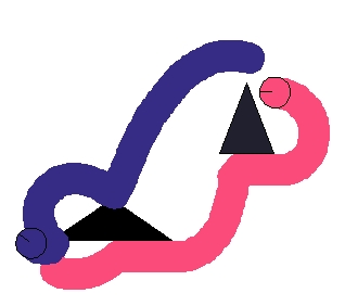
`Rock Path' (4 objects, 83 frames) - In this cast, Two rock objects act as attractors
for the two cross-wired kit-bugs.
But the impenetrability of rock can be a problem. On
colliding with a lump of rock, a bug is automatically
`swerved' to one side (provided the setting for
`autoSwervingAmount' is a non-zero value). Although this
does not affect
`Rock Path' too badly, it can easily produce
ugly discontinuities in the image. In this situation it may
be better to use `mud'. Mud is similar to rock in that it
cannot be moved. But its penetrability means that collisions
are no longer a problem.
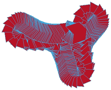
`The Saddle' (4 objects, 288 frames)
`Upside Down Cleavage'
is cast from a similar setup. It uses
a large dollop of mud and a single bug. The bug is attracted
to the mud but on entering is firmly deflected to the left.
The result is a `fluttering' motion which gradually
encircles the arena.
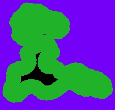
`Upside Down Cleavage' (2 objects, 155 frames)
Cast from a slightly modified setup, `Pop' uses a `pile' of
copies of the original mud object and a star shaped bug.
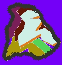
`Pop' (7 objects, 211 frames)
`Shattered' on the other hand uses three blobs of fairly
thick mud together with a couple of cross-wired kit bugs
which have been given dart-like shapes. The shell colors of
both bugs have been made invisible so as to emphasise the
starburst effect produced when orbiting a mud object.
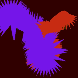
`Shattered' (5 objects, 100 frames)
`Slinky Balls' is a variation on the theme further
demonstrating use of bugs with invisible bodies.
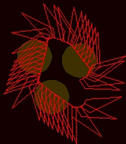
`Slinky Balls' (4 objects, 38 frames)
Collecting debris
Debris is like rock in that it cannot be penetrated. But it
can be `pushed' around the arena. Debris objects are useful
for BugArt purposes because, like bugs themselves, they
leave a trail when moved. In `Squeeze Out', a large number
of round, blue debris objects have been placed in the middle
of the arena. A single yellow bug with an invisible shell
color is then `set loose'. As the bug pushes towards the
centre of the pack, the mud objects are pushed to one side,
leaving trails as they go.
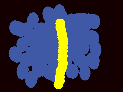
`Squeeze Out' (33 objects, 705 frames) - In this cast, a large number of debris objects are
pushed aside as the yellow bug moves forwards. A black
background has been used to emphasise the yellow/blue
contrast.
The slightly chaotic trajectories of debris trails contrast
with the smoothly curving and straight-line trails we
generally obtain from kit-bugs. Their presence creates a
sense of disorder which may be lacking in images constructed
purely from active-bug trails.
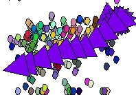
`Reluctant Sweets' (69 objects, 151 frames)
`Reluctant Sweets' presents a similar effect but with a
lighter image and randomly-colored debris. The large
triangular bug moves through a `cloud' of randomly colored
debris, pushing the objects to one side as it does so.
Sensor filters
With rock, mud and debris brought into play, it is often
desirable to control the reactions that bugs have to
different types of object. For example, we may want to
modify a kit-bug so that it will only be attracted to
passive objects and not to other bugs. (This is what we
needed to do in order to create the `Different Curves'
image earlier on.)
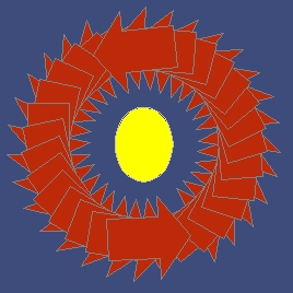
`Arrow Eye' (3 objects, 15 frames) - In this simulation, two arrow shaped kit-bugs use
filtered sensors so as to avoid responding to each other.
When first created, kit-bugs are equipped with what are known
as `proximity sensors'. These respond indiscriminately to
everything in the arena. They generate a signal which reflects
the proximity of the nearest object in the arena regardless of
what that object actually is. By adding filters to such
sensors, however, it is possible to refine their sensitivity.
[proximity]
[proximity [type rock]]
[proximity [color yellow]]
[proximity [color blue][shape triangle]]
[proximity [name rock3]]
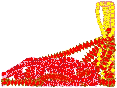
`Selective Chase' (3 objects, 584 frames) - An image showing unusual kit-bug dynamics resulting
from use of sensor filters. Each bug was endowed with a
tendency to approach bugs of one color but flee from bugs of
another.
Endowing all three bugs with oversized wheels produces the
remarkably different `Behind the Facade', illustrating the
general principle that in BugArt it is difficult to predict
what lies `just around the corner' in a particular setup.
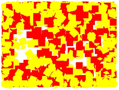
`Behind The Facade' (3 objects, 1031 frames)
[proximity [shellColor green]]
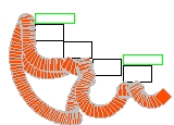
`Upstairs Downstairs' (7 objects, 288 frames)
Pause
Illustrating some of the possibilities of methods described in
this chapter, the pause gallery presents a range of images
cast using highly contractive samplings. In `His Dark
Pyjamas', the underlying simulation comprised a number of
hand-drawn kit bugs `running amok' among a set of hand-drawn
debris objects. `Depths of Mud' was cast from a similar setup,
but in this case using a single, lump of hand-drawn, invisible
mud. The differently-flavoured `Suspended Mud' benefits from a
pseudo-3-dimensional background effect built-up using com-bug
shell trails.
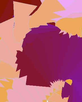
`His Dark Pyjamas' (2 objects, 364 frames) - A selection of hand-drawn kit-bugs interacting in a
`soup' of hand-drawn debris objects yields this image, cast
from a small portion of the arena.
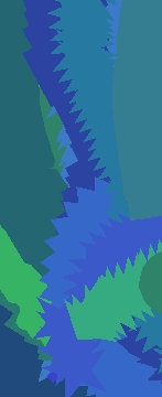
`Depths Of Mud' (15 objects, 119 frames) - A contractive cast focussing on a small
detail from a simulation involving a number of hand-drawn
kit bugs interacting around a `pool' of low-solidity mud.
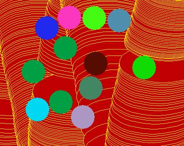
In this cast, a scattering of mud objects with
negligable solidities modulate the behaviour of a large
com-bug `bouncing' across the arena.
Up to this point, BugArt has been a little like letting off
fireworks: we set out the bangers, rockets and catherine
wheels (or at least the mud, bugs and rock), we light the
blue-touch paper and stand well back. The process has been a
strictly `hands-off' activity. But it doesn't have to be
like that. BugWorks provides a range of ways in which the
bugartiste can work `hands-on'. By getting more directly
involved in the image-generation process, effects can be
achieved which may be difficult to produce any other way.
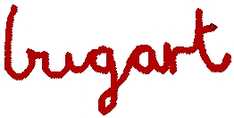
`Bugart' (1 object, 885 frames) - With trails switched on, hand-drawn images can be
produced by dragging objects around the arena.
BugWorks will let you carry out any action while the
simulation is running. This means that you can interact with
a `live' arena. Having started a simulation running, you can
add a new piece of debris, change the color of the
background, add a sensor to a bug, change the width of a
rock, or anything else that appeals. Any changes made will
directly affect the image. If you move a rock from one place
to another, for example, the image will show the relevant
trail that you created in doing so.
Follow-me brush strokes
A quick way to get started with hands-on-top creativity
involves setting up a simulation in which a set of standard
bugs chase after an object that you move around the arena by
hand. I call this the `follow-me' technique. Follow-me
images are fun to produce and the method vastly extends the
range of patterns that can be achieved.
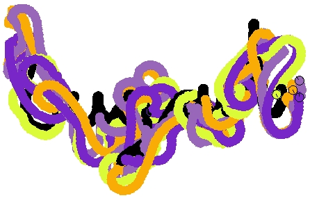
`Spagarti' (5 objects, 670 frames) - A hands-on-top image in which cross-wired kit-bugs
pursue a target that is moved around the arena by hand.
Note that it is best to take advantage of the impenetrable
property of rock in follow-me experiments. If you use a mud
object, the bugs will tend to move across it while the
simulation is running, making grabbing difficult. Another tip
for follow-me creativity: if you hold down the CTRL key while
you drag the target around, the bugs will match their speed
with the motion of the object. This allows you to keep a
tighter rein on developments.
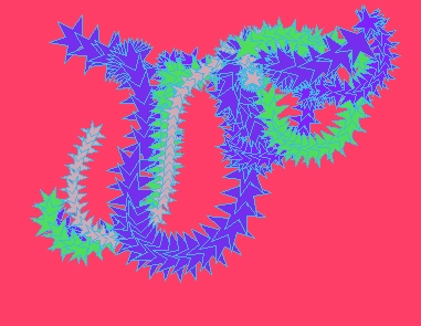
`Invisible Target' (5 objects, 479 frames) - A follow-me image illustrating use of an invisible
target.
For bigger, brighter variations on this theme, just add more
kit-bugs in a greater variety of shapes, sizes and colors.
As always, the easiest approach involves using the Modify
window to inject variety. `Pulse Chasers' users star-shaped
bugs and a target which `pulses` from left to right.
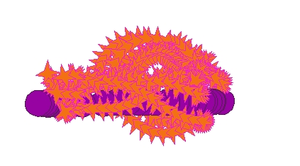
`Pulse Chasers' (5 objects, 113 frames) - A follow-me image in which a visible target is
moved from right to left across the arena.
Color bending
BugWorks provides color sliders for manipulating the color
of selected objects. Like all other components of the user
interface, these can be used while the simulation is
running. This means that we can use them to `bend' the color
of bugs and other objects while they are moving around the
arena.
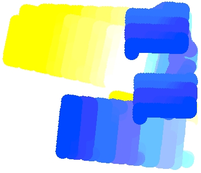
`Kenwood Bender' (3 objects, 1631 frames)
Color bending can also be applied with kit-bugs. The
familiar tail-chase image produced by three kit-bugs
pursuing each other around the arena becomes more
interesting if the colors of the bugs are updated using the
sliders while the chase is ongoing.
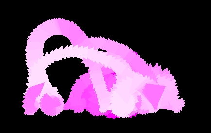
`Depressed Hoover' (3 objects, 388 frames) - Using the color sliders, the color of bugs can be
modified while the simulation is running. In this image, the
green slider was used to create a range of magenta shades.
`Sex Alert' is based on an interaction between three
kit-bugs with the color sliders being used to slowly bring
out a red shade in just one of the bugs. The unusual
dynamics were achieved by using the Modify window to
randomly reset the sizes of all the wheels. (This involved
using the window with `parts' and `size' checked.) The bug
shells have been made invisible so as produce a more
`squirted' effect.
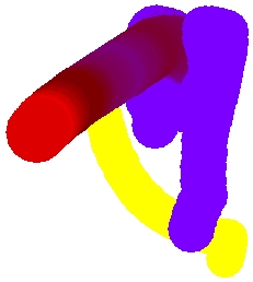
`Sex Alert' (3 objects, 66 frames) - An image illustrating the use of color sliders to
vary the shade of a single object.
For a gentler, more rural effect consider `Pine Cone Love'.
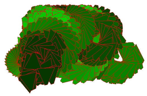
`Pine Cone Love' (3 objects, 368 frames) - A simple cone shape was defined
and selected in three kit-bugs. The shape modulates the
normal, kit-bug interaction due to the different types of
collision which are now possible. Hands-on color-bending was
used to vary shades.
Bug windows as control panels
Hands-on-top creativity depends on the functionality
provided by the user interface. The follow-me technique
exploits the fact that objects can be dragged around the
image while the simulation is running. The color-bending
technique exploits the potential of the color sliders. Many
other opportunities are offered by the kit-bug window. This
window shows the bug's components along with a tool bar
(accessed with the `Show tools' button) for manipulating
those components. As usual, everything in the window can be
manipulated while the simulation is running. In effect, the
window can therefore be used as a kind of control panel for
the bug.
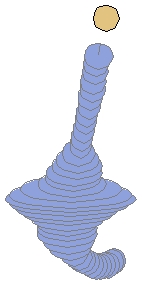
`Inner Tube' (2 objects, 53 frames) - Use of the Resize tool in a bug window allows for
dynamic reshaping.
The Resize tool can also be used to resize parts. If the
bug is transparent its parts will be visible in the main
window and any changes of part dimensions will change the
`brush pattern' produced by the bug. `Iris Cutter' features
an enlarged standard bug circling some mud, while one its
sensors is slowly stretched out in the corresponding window.
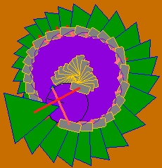
`Iris Cutter' (9 objects, 51 frames) - An image illustrating the use of the Resize tool
to dynamically modify the size of a part.
Parts in the bug's window can also be repositioned. Assuming
the bug is transparent, this is another good way to alter
the bug's `footprint' in the image. `Breast Kicks'
illustrates the possibilities.
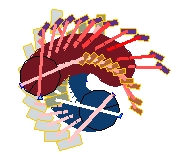
`Breast Kicks' (14 objects, 100 frames) - In the simulation from which this image was cast,
the position of the brown bug's right sensor was manipulated
as the run proceeded.
Cast from a similar setup but rather more complex, `Dancing
Cobras' relies on the manipulation of wheel position to
produce a splaying effect. With the simulation running, the
right wheel of the dark-colored bug was slowly dragged from
left to right. The resulting motion produces the `embankment'
effect in the trail while the natural tendency of the bugs to
curl around each other creates a vertical iteration of
twisting bars.
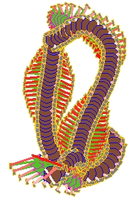
`Dancing Cobras' (18 objects, 123 frames) - Hands-on manipulation of wheels was used in this
simulation to produce a rhythmic splaying action.
The striping effect in `Dancing Cobras' benefits from
inclusion of a range of red shades. This results from the
fact that, with a transparent body, any sensor-wheel channel
is drawn in a shade of red corresponding to the amount of
activation carried by the channel. For greater control over
this, you may want to re-define the range of shades in which
channels are drawn. As previously explained, this is done by
updating the `activationColorRange' value in the Settings
dialog.
Dynamics bending
Changing part positions can have interesting secondary
effects if, as is the case with the cross-wired kit-bug,
those parts are sensors and their functionality depends on
their position. Remember that the behaviour of a kit-bug
depends on the way in which the sensors connect to the
wheels. If the connections are crossed, the bug will tend
to approach the closest object. If the connections are
uncrossed, the bug will tend to move away from it.
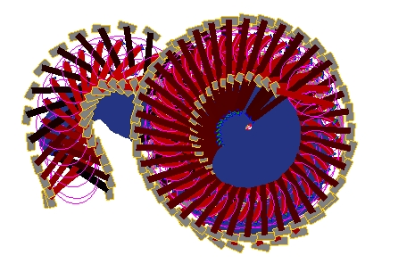
`No Farthing' (8 objects, 330 frames) - A cast showcasing the effects of in-simulation
part-dragging.
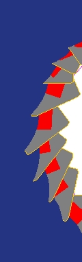
`No Farthing Cast2' (8 objects, 330 frames) - A more contractive cast, focussing on the boundary
between the two trails.
Use of groups
The possibilities for creating novel dynamics are particularly
good when hands-on manipulation is used with groups. To create
a group, first select the bugs you want to included. You can
use the selection box to do this. Or you can select the
members one by one. But remember to hold down the SHIFT key so
as to accumulate selections.
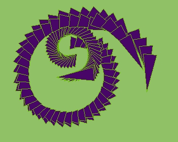
`Its Rude To Expand' (3 objects, 45 frames) - The dilation effects in this image were achieved
by placing three bugs in a group and then using the Resize
tool from the group window to dynamically modify bug
length.
`Group Hug' and `Degroup Hug' were cast from a similar
setup. In the case of `Group Hug', sensor positions were
manipulated to produce varying dynamics.
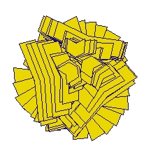
`Group Hug' (3 objects, 592 frames) - Dynamic modification of sensor position impacts the
dynamics of the group.
With the group cancelled and attributes randomised to
produce a more visually diverse effect, the simulation
yields the different `De Group Hug'.

`De Group Hug' (3 objects, 41 frames)
Shape groups
For BugArt purposes, group-related effects are often more
conveniently achieved through use of a named shape. Once a
shape has been created and named, any bug can be set to use
that shape by specifying the relevant name in its Properties
dialog. Subsequently, any change made to the shape, in
whatever context, will affect the shape of all users of the
shape. The name thus defines implicitly a `shape group'. The
advantage for the bugartiste is that the bugs in this type
of group are able to have different values for key visual
attributes such as color and size.
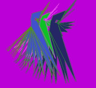
`Bugs Of Paradise' (3 objects, 83 frames)
For the traditional artist, this type of hands-on approach
may feel more natural than some of the other techniques
we have explored. Using a bug window as a `control panel'
for purposes of manipulating a set of on-screen objects is a
bit like using a texturing tool tool in a
modern art package. Using color sliders to `bend' the color
of an object as it moves along a trajectory is similar to
dynamically altering a gradient definition. Indeed there is
nothing to rule out using the system exclusively in this
way, as a package of object-oriented drawing and texturing
tools.
Pause
And so to the penultimate pause gallery of the book. In this
case the presentation is made up of a selection of images all
of which share the property of having involved some form of
hands-on activity.
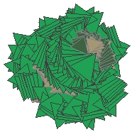
`Cushion Of Death' (3 objects, 479 frames) - This image was constructed using dynamic
part-resizing and triangular bugs. The form of `tail chase'
obtained conjures up an impression of a 3-dimensional
object.
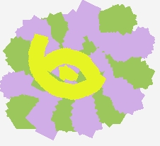
`Wallpaper Of Yin' (3 objects, 500 frames) - In this image, randomisations of `position' and
`heading' were applied (via the Modify window) while the
simulation was running so as to repeatedly destabilise the
dynamics and maximise coverage of the arena.
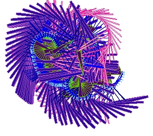
`Overload' (14 objects, 97 frames) - An image featuring perhaps a little too much
visual activity. Using group-based manipulation techniques,
it is easy to generate clutter.
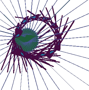
`View From The Top' (2 objects, 36 frames) - Another image illustrating the effects which can be
achieved by hand-manipulation of parts.
Earlier in the book, we saw how com-bugs could be
controlled using `move', `turn' and `set' commands. In this
chapter we will examine some other commands that can be
used and look at the opportunities for experimentation. The
complete set of commands which can be used in BugWorks is
called `BugScript'.
Advanced uses of `set'
A certain amount of attention has already been given to the
`set' command. We've seen how it can be used to set new
values for a bug's attributes. For example
set bug.color = red
set num = 2
  set num = 4
  set product = num * num
   set num = 4
   print hello num
  set num = bong
  print hello num
  set sentence = a number of words
  print sentence
   set name = what is your name ?
   print name
  set val = 2 + 4 * 3 + (12 / 4)
  print val
  set val = 2 + 4 < 3 * 6
  print val
Random numbers
When using the `set' command we often want to store a
randomly chosen number in a variable. This can be done using
a `random' variable, just the same way we did when
implementing random-sized moves and turns. For example
set x = random15
set x = random3.0
set x = random3
   turn random100 - 50
   move 10

`Drunk Again' (1 object, 161 frames) - A random walk.
In BugWorks, turns are implemented by adding the turn value
to the bug's heading. So a negative turn value implies a
turn to the left while a positive value implies a turn to
the right. A bug whose heading is 180 degrees (due south)
executing a turn of -90 degress ends up with a heading of 90
degrees (due west). Following a turn of 90 degress, on the
other hand, the bug ends up with a heading of 270 degrees
(due east).
set bug.width = bug.width + random10 - 5
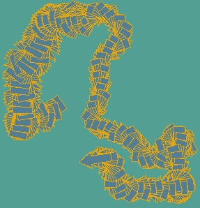
`Drunken Dilation' (1 object, 719 frames) - A cast derived from a simulation combining a random
walk with continuous, random dilation of width.
Random colors
As we've seen, the color of any object in BugWorks can be an
RGB value, i.e. a set of three values in the range 0-255,
specifying the red, green and blue intensity respectively.
To endow the bug with a randomly selected color, then, we
can use a `set' command in conjunction with three random
values:
set bug.color = random255 random255 random255
   set bug.color = random255 random255 random255
   set bug.heading = random360
   move 50
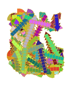
`Dart Storm' (1 object, 718 frames)
Reducing the size of the `move' and introducing an oval
bug-shape produces the calmer `Gums'.
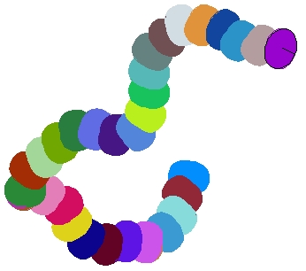
`Gums' (1 object, 234 frames)
Often, when generating random colors, there will be a desire
to generate particular shades. One way to achieve this is to
adjust the ranges in which the random numbers are generated.
For instance, to generate some sort of dark red color we
might use
set bug.color = random100 random20 random20
set bug.color = 200 + random55 200 + random55 200 + random55
   set r = 200 + random55
   set g = 200 + random55
   set b = 200 + random55
   set bug.color = r g b

`Light Gums' (1 object, 81 frames) - An image illustrating the use of constrained
randomisation to achieve a sequence of light shades.
Having to introduce special variables in order to get control
of individual intensities is long-winded, but the system's
suffix mechanism for color intensities does make things a
little easier. An `R`, `G' or `B' may be attached to the end
of any color variable, so as to get at the red, green or blue
intensity individually. To access the green intensity of the
bug's color, for example, we use
bug.colorG
set bug.colorG = 100
  set bug.colorG = random100
  set bug.colorB = 100 + random100
  set bug.colorR = 200 + random55
  move 100
  set bug.heading = random360
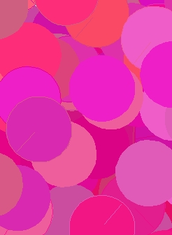
`Class Of Pink' (1 object, 481 frames) - An image cast from a simulation in which a com-bug
repeatedly resets its color intensities within constrained
ranges.
The `init' command
Like the `set' command, the `init' command sets a variable
to a value. However, `init' commands are only executed once,
at the start of any run. This means they can be used to
initialise variables or attributes.
   init bug.X = 10
   init bug.Y = 10
init bug.heading = 180
The `if' command
Like any programming language, BugScript implements the
conditional `if' command. This is an odd command because it
doesn't do anything directly. Rather it executes a second
command depending on the truth of an expression. For example
if 2 = 2 print yes
if 2 = 5 print yes
  set x = 2
  if 2 = x print of course
  set x = 2
  set y = 4
  if (x + 2) < (y + (x / 3)) print yes
Basic scheduling using a counter variable
The simplest program for a com-bug program is just a
sequence of `turn' and `move' commands. The program says
what the bug should do in each cycle of the simulation. It's
a case of `everything every time'---every instruction in the
program is executed in every cycle of the simulation. But
using BugScript commands such as `if' and `goto', we can get
beyond this and start making use of programs which schedule
different behaviours to happen at different times.
    move 5
    turn 2
turn 180
   move 5
   turn 2
   move 5
   turn 2
   move 5
   turn 2
   move 5
   turn 2
   move 5
   turn 2
   move 5
   turn 2
   move 5
   turn 2
   move 5
   turn 2
   move 5
   turn 2
   move 5
   turn 2
   move 5
   turn 2
   turn 180
   init t = 0
   set t = t + 1
if t = 30 turn 90
20 % 10
14 % 10
  init t = 0
  set t = t + 1
  move 5
  turn 2
  if t % 30 = 0 turn 180

`Curve Reversal' (1 object, 307 frames) - An image illustrating the use of a counter variable
to schedule a trajectory-reversal in every 30th simulation
cycle.
If we want perfect trajectory reversal, then we need to
reverse the angle of turn each time we reverse direction.
Again, this requires use of a variable:
  init a = 2
  init t = 0
  set t = t + 1
  move 5
  turn a
  if t % 30 = 0 turn 180
  if t % 30 = 0 set a = -a
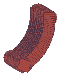
`Perfect Curve Reversal' (1 object, 1822 frames) - A bug requires a certain amount of room to execute
a 180-degree turn. The net effect is that, in the
curve-reversal simulation, curves are gradually built up on
the side towards which the bug makes its turn.
The bigger `if', the flexible `goto'
The simulation of curve-reversal required use of a counter
variable to count simulation cycles. By applying `if'
commands to the value of this variable (in fact to the
remainder produced by dividing it by the required interval)
we were able to schedule the relevant actions to happen at
the right moment. But what happens if we have a large
number of actions which need to be scheduled at a
particular time? Is it going to be necessary to precede
each command with an identical `if' command?
  init a = 2
  init t = 0
  set t = t + 1
  move 5
  turn a
  if t % 30 != 0 goto end
  turn 180
  set a = -a
  init a = 2
  init t = 0
  set t = t + 1
  move 5
  turn a
  if t % 30 != 0 goto doobydoo
  turn 180
  set a = -a
  setpos doobydoo
  init a = 2
  init t = 0
  set t = t + 1
  move 5
  turn a
  if t % 30 != 0 goto end
  set a = -a
  turn 170
  set bug.colorG = bug.colorG - 5
  set bug.size = bug.size - 1
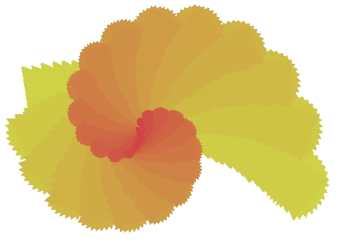
`Unfurling' (1 object, 3225 frames) - An image cast from a simulation derived by applying
some minor modifications to the curve-reversal program.
Further changes may or may not yield interesting results:
  init t = 0
  init a = 2
  set t = t + 1
  move 5
  turn a
  if t % 30 != 0 goto end
  turn 190
  set bug.colorG = bug.colorG - 5
  set bug.length = bug.length + 1
  set a = -a
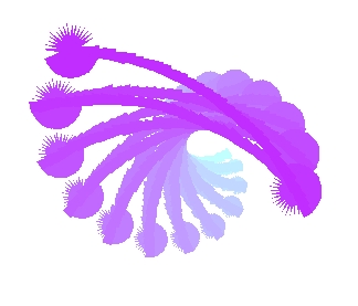
`Pot Plant Launcher' (1 object, 2393 frames) - Cast from the same setup as
`Unfurling', this shows
a bug in an expanding trajectory-reversal cycle, with length
increasing and green-intensity decreasing.
Looping with `setpos' & `goto'
Though rarely of use in BugArt applications, the `goto'
command can also be used for explicit looping, i.e., for
getting the computer to explicitly repeat a sequence of
commands. By placing a suitable `setpos' command at the
beginning of the code we want to repeat, and a `goto' at the
end, we can make the computer keep jumping back and going
over the same sequence again. For example, here is a little
program which prints out all the numbers from 0 up to
20 by repeatedly executing the commands between `setpos
loopstart' and `goto loopstart'.
  init x = 0
  setpos loopstart
  print x
  set x = x + 1
  if x < 21 goto loopstart
if x < 21 goto loopstart
goto loopstart
The twist setup
The trajectory-reversal examples show how we can make single
com-bugs generate complex geometric patterns without the
need for any interaction. Those examples made use of
movement around the arena. It is also possible to generate
patterns with bugs that stay in one place.
turn 45
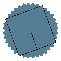
`Box Twist1' (1 object, 250 frames)
Changing the `shellColor' of the bug to something that
leaves a trail (e.g., `red'), we get `Box Twist2' and the
beginnings of a pattern.
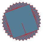
`Box Twist2' (1 object, 144 frames)
Continuing on, we can make use of a toggle variable to make
the bug change its size as it spins:
   init d = 1
   turn 9
   set bug.size = bug.size + d
   if bug.size < 5 or bug.size > 100 set d = -d
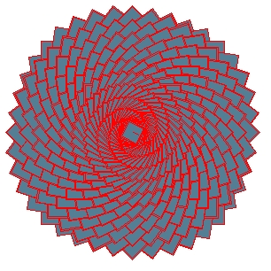
`Box Twist3' (1 object, 342 frames)
Variations on this setup are easy to generate. We can change
the color of the bug or its shell using `set' commands
within the program. We can also modify the behaviour by
slightly altering the numbers that are used as
initialisations and thresholds. Changing the `turn' angle,
for instance, changes the pattern in interesting ways, as
does changing the `init' command so as to give a different
starting value to `d'. Using an orange-based color scheme
and the commands `turn 13' and `init d = 4' produces `Box
Twist4'.
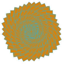
`Box Twist4' (1 object, 101 frames)
Another way to progress this is to have the program vary
features of the bug in synchronisation with the dilation.
For example, we might focus on varying color:
  init d = 2
  turn 8
  set bug.size = bug.size + d
  set bug.colorG = bug.size
  if bug.size < 5 or bug.size > 100 set d = -d
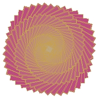
`Box Twist5' (1 object, 175 frames)
To make the color variation a little more prominent, we can
set the shell color to be `invisible' and amplify the color
variation by setting the green intensity to be three times
the current size:
set bug.colorG = bug.size * 3
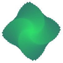
`Box Twist6' (1 object, 69 frames)
A further variation is obtained by arranging for the shell
color to be varied along with the color and size:
  init d = 2
  turn 8
  set bug.size = bug.size + d
  set bug.colorG = bug.size * 3
  set bug.shellColorR = bug.size * 2
  if bug.size < 5 or bug.size > 100 set d = -d
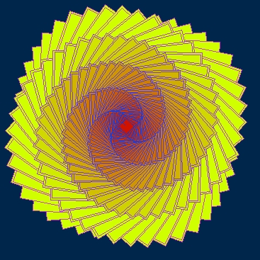
`Box Twist7' (1 object, 177 frames)
With this cast we are getting towards something that is
visually quite interesting. But many avenues remain
unexplored. We have made no use of the possibilities of
lateral motion, for instance. The bug merely rotates on the
spot, shrinking and expanding as the simulation continues.
 init d = 5
 init-bug.size = 23
 turn 15
 set bug.size = bug.size + d
 set bug.colorG = bug.size * 3
 set bug.shellColorR = bug.size * 2
 if bug.size < 5 or bug.size > 70 set d = -d
 if bug.size < 5 move 500
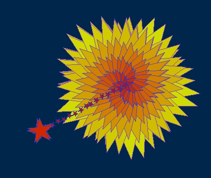
`Star Birth' (1 object, 67 frames)
From the same setup (but using different cast settings), we
get `Ecstatic', generated using a triangular bug and a much
longer simulation sequence. Note how the slight asymmetries
in the bug's rotation means that the move command is
executed at different orientations. The overall effect is of
the bug `jumping' from position to position, executing one
complete cycle of expansion and contraction at each site
before finally returning to its starting position.
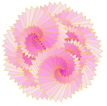
`Ecstatic' (1 object, 955 frames) - A rotating, dilating, triangular
com-bug programmed to execute a forwards jump when its size
reaches a minimum threshold. Color-changing commands cause
the color to vary in synchronisation with size.
Contractive casting
With such complex simulations, images based on a full view
of a complete simulation run can be visually overwhelming.
In this situation it may be better to cast the image
from a small sample, showcasing just one aspect of the
underlying behaviour. As we have seen, such samples are
easily generated using the BugWorks Movie facility
(accessed via the Movies button).
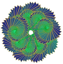
`Triangle Twist5' (1 object, 981 frames) - An image cast from an entire triangle-twist
simulation.
To simplify the image, one might consider casting from a
short initial sequence of the run, as in `Triangle Twist3'.
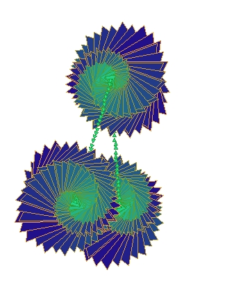
`Triangle Twist3' (1 object, 434 frames)
As an alternative, the cast might use the zoom feature to
focus on a small region of the arena, as in `Triangle
Twist4'.
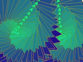
`Triangle Twist4' (1 object, 318 frames) - An image cast from a very small region of the
arena.
Highly contracting samplings such as these can produce
surprisingly different visual effects---effects which seem
to be only distantly related to the original
simulation. For example, consider `Custom Twist1'. This was
derived from the same setup but using a hand-drawn bug shape
with an invisible shell.
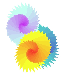
`Custom Twist1' (1 object, 258 frames)
Taking a cast from a small region on the boundary between
two stars yields the `sunrise' effect of `Box Twist8'.
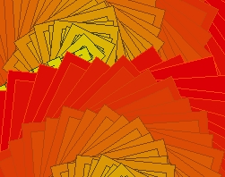
`Box Twist8' (1 object, 306 frames)
As an extreme example of contractive casting, consider
`Mist
Twist'. This uses the simulation sequence that builds the
dark blue star in `Custom Twist1', focussing on a tiny
region just above the star's center.
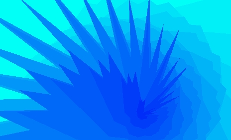
`Mist Twist' (1 object, 205 frames) - Illustrating the effects of contractive sampling,
this image was constructed using a sequence of around 30
frames and a region representing less than 1/100th of the
arena surface.
Programmed interaction
The setups we have been looking at use a single bug. All the
visual effects therefore result from behaviour the bug
produces spontaneously. Often these involve some sort of
dilation combined with some sort of rotational movement, as
in `Perfect Hernia'
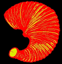
`Perfect Hernia' (1 object, 441 frames)
or the closely related `Shell Wrap'.
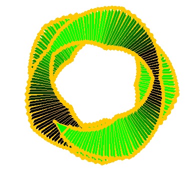
Often, though, we want to make use of interaction. We want
to see what sort of effects can be obtained when one bug's
behaviour is affected by that of another.
set bug.size = bug.fred.size
set bug.color = obj.rock1.color
set bug.Y = bug.nearest.Y
Sensing proximity and direction
For programs in which we want one bug to react to the
proximity or direction of another, we can make use of the
`distance' and `direction' variables. The `direction'
variable always contains the compass bearing of the relevant
bug. So
set bug.heading = bug.nearest.direction
set bug.heading = bug.nearest.direction + 180
set bug.colorG = bug.nearest.distance
set bug.shellColor = obj.arena.color
set obj.arena.color = cyan
goto end
goto start
Examples from the `wriggler' setup
With these special variables to hand, there is no shortage
of ways in which we can make a com-bug responsive to its
environment and the behaviour of the objects around it. We
are all set to explore ways of exploiting interaction
between com-bugs.
  init d = 0.5
  init limit = 7
  init a = 0
  set a = a + d
  if a > limit or a < -limit set d = -d
  turn a
  move 3

`Basic Wiggler' (1 object, 372 frames)
Of the seven commands, it is the two at the end which
actually generate the motion. To understand how the
program works, start at the end and work back. The `move'
command produces a small forwards move of a fixed size while
the `turn' command produces a turn whose angle is fixed by
the value of the variable `a'. The number of degrees turned
is whatever the current value of `a' is.
set bug.size = obj.nearest.distance / 5
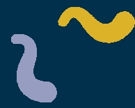
`Wriggling Dilation' (2 objects, 163 frames) - An image cast from a simulation in which bugs
dynamically reset their size depending on their proximity to
each other.
For best results, we should also pay attention to color. A
simple approach would be to add a second `set' command which
applies the same approach to the bug's color attribute as
has already been applied to its size. For example, we might
use
set bug.colorG = obj.nearest.distance
set bug.colorR = obj.nearest.direction
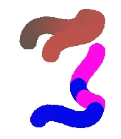
`Bouts Of Depression' (2 objects, 549 frames) - With color reset as a function of the direction of
the nearest bug, sudden changes in shade will occur as the
relative heading changes between 0 and 359.
Instead of using the `direction' variable, we are better off
using either the `elevation' or `transition' variable. For a
given bug, these show how far ahead the bug is along a
particular axis. The `elevation' variable shows how far
ahead the bug is in the northwards direction. The
`transition' variable shows how far ahead it is in the
westwards direction.
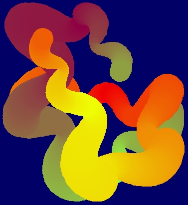
`Snakes Behaving Like Dogs' (2 objects, 798 frames) - In this cast, color is reset in each bug depending
on the elevation of the other bug.
To implement this effect, use a set command to set the color
intensity value directly from the either the `elevation' or
`transition' variable:
set bug.colorG = obj.nearest.elevation
set bug.colorG = (obj.nearest.deviation / 180) * 255
  init d = 0.5
  init limit = 7
  init a = 0
  set a = a + d
  if a > limit or a < -limit set d = -d
  set bug.size = obj.nearest.distance / 4
  set bug.colorG = (obj.nearest.elevation / 180) * 255
  turn a
  move 2
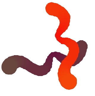
`Cellosunder' (2 objects, 327 frames)
These com-bug casts have a noticeably different character
from those generated using either kit-bugs, or spontaneous
com-bugs. There is a clear interactive element here, as
there is in any kit-bug chase. But the effect here does not
involve changes of direction. Rather, it involves changes of
size: the bug's contract as they draw near to each other
and expand as they move away. At the same time they are
changing hue as a function of their spatial relationship on
the north/south axis.
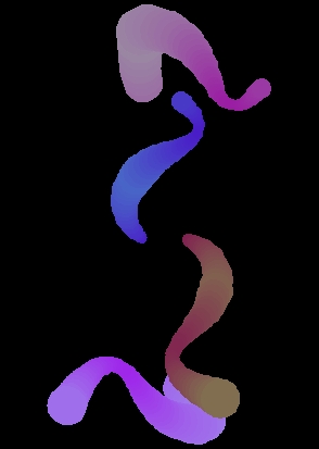
`Geisha' (4 objects, 178 frames)
As ever, we have the possibility of re-generating the image
from different starting conditions. And the
results can be quite surprising. As an illustration,
consider `The Blessing'. This was cast from the `Geisha'
setup but using just two box-shaped bugs and different
initial colors. Again, the image is based on a very short
simulation sequence.
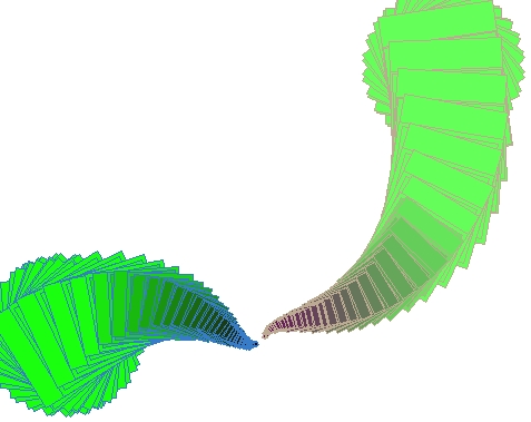
`The Blessing' (2 objects, 137 frames)
A personal favourite from this batch of casts is
`The Kiss'.
This re-uses the `Geisha' setup but returns to the use of
just two bugs. Again, different initial colors have been
applied and the image has been cast from a short simulation
sequence.

`The Kiss' (2 objects, 281 frames)
BugScript programming: a footnote
The set of commands that can be used with com-bugs is known
as `BugScript'. And though it may not be obvious, BugScript
is a actually a simplified programming language for
computers. Unlike most programming languages, BugScript is
tailored to a very specific task---namely the control of
bugs. But it does have many of the properties of a true
programming language and can even be used (at a stretch) for
traditional, data-processing purposes.
Tied strings
We have seen already that BugScript allows use of strings of
characters, i.e., words, phrases and sentences. For example,
consider the `hello world' program, which simply prints out
`hello world'. This is the first program to be attempted in
any programming language. In BugScript it is just
print hello world
set x = 2
print foo~x
  set y = grunge
  set z = bongos
print y~shack~z
  set foo1 = baz
  set i = 1
  print foo~i
  set a1 = foo
  set a2 = baz
  set a3 = dong
  set a4 = bing
  set a5 = goo
  set i = 1
  setpos loop
  print a~i
  set i = i + 1
  if i < 6 goto loop
Array processing
Using a variable-based `array' and a setpos/goto pair we can
create a looping process which will process all the data
stored in that array. For example, this example sums the
values stored in the `array' and prints out the total.
  init a1 = 8
  init a2 = 93.623
  init a3 = 0.0003
  init a4 = 967544
  init i = 1
  init total = 0
  setpos loop
  set total = total + a~i
  set i = i + 1
  if a~i > 0 goto loop
print The sum of the i values is total
Processor implants: the hybrid kit/com-bug
With the full power of BugScript to hand, there are many new
things we can do. We can write much more complex com-bug
programs for one thing. We can also start to exploit the
possibilities of the `processor implant'. In this technique,
we insert a programmable component into a kit-bug so as to
turn it into a hybrid kit/com-bug. This approach
gives us the best of both worlds, with regard to
functionality and flexibility.
set bug.colorG = bug.nearest.elevation
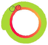
`Elevated Chase' (2 objects, 78 frames)
For better results, add similarly-programmed processors to
buth bugs (or put the bugs in a group). In the case of the
present setup, this produces `Elevated Chase2'.
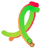
`Elevated Chase2' (2 objects, 96 frames)
For best results, use the Modify window to apply further
randomisation of attributes. `Abduction Threat' exemplifies
what can be achieved.
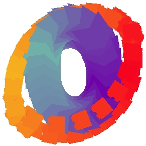
`Abduction Threat' (2 objects, 86 frames)
For purposes of eliminating all trace of the familiar
`tail-chasing' dynamics, a randomising `turn' command
inserted into the processor may be of use. For example, the
command
turn random100 - 50
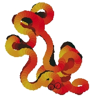
`Furenze' (2 objects, 385 frames)
Choosing how to further develop a setup involving hybrid
kit/com-bugs is really a matter of personal choice. Dilation
effects are easily introduced and will often produce
interesting results. The command sequence
   set bug.width = bug.width + 10
   if bug.width > 100 set bug.width = 10
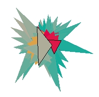
`Furenze2' (2 objects, 64 frames)
Dilation effects can be applied to both bugs at once. We can
also arrange to have length vary inversely with width,
producing a kind of `squelching' body mutation.
  set bug.width = bug.width + 10
  set bug.length = 100 - bug.width
  if bug.width > 100 set bug.width = 10
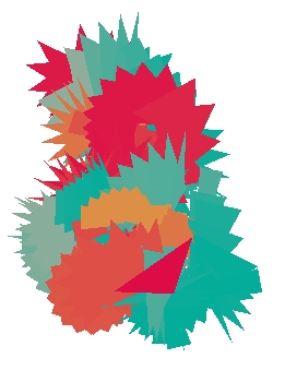
`Furenze3' (2 objects, 169 frames)
The same setup with box-shaped bugs and a new color scheme
yields `Exterminate'.
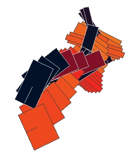
`Exterminate' (2 objects, 22 frames)
It takes only a small change to the processor programs to
generate significant visual alteration. `The Fate of Onion
Sellers' illustrates the point. Like `Exterminate' this was
generated from the setup used for `Furenze3' but with
modified variable values, oval bugs, invisible shells and
differently initialised colors.
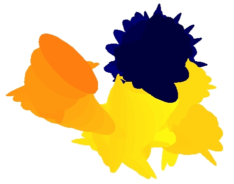
`The Fate Of Onion Sellers' (2 objects, 80 frames)
It's tempting to continue this process of experimentation in
the hope of achieving ever more visual diversity. For
example, we could attempt to make more use of the motional
functionality of the processor implants, perhaps adding
commands to make the bugs produce specific movements in
specific parts of the arena (or when in a specific
relationship with another bug). But at this level of
complexity we are already dangerously close to the point at
which further additions will probably yield diminishing or
negative returns. With BugArt it is always easy to add more.
But there comes a point at which `more' produces `less'.
Beyond this point, it is not be long before `more' becomes
`total chaos.' One of the key skills for the bugartiste is
knowing when to stop.